Summarise the results of node-splitting models
Source:R/nma_nodesplit-class.R
summary.nma_nodesplit_df.RdPosterior summaries of node-splitting models (nma_nodesplit and
nma_nodesplit_df objects) can be produced using the summary() method, and
plotted using the plot() method.
Usage
# S3 method for class 'nma_nodesplit_df'
summary(
  object,
  consistency = NULL,
  ...,
  probs = c(0.025, 0.25, 0.5, 0.75, 0.975)
)

# S3 method for class 'nma_nodesplit'
summary(
  object,
  consistency = NULL,
  ...,
  probs = c(0.025, 0.25, 0.5, 0.75, 0.975)
)

# S3 method for class 'nma_nodesplit'
plot(x, consistency = NULL, ...)

# S3 method for class 'nma_nodesplit_df'
plot(x, consistency = NULL, ...)
Arguments
- consistency
Optional, a
stan_nmaobject for the corresponding fitted consistency model, to display the network estimates alongside the direct and indirect estimates. The fitted consistency model present in thenma_nodesplit_dfobject will be used if this is present (seeget_nodesplits()).- ...
Additional arguments passed on to other methods
- probs
Numeric vector of specifying quantiles of interest, default
c(0.025, 0.25, 0.5, 0.75, 0.975)- x, object
A
nma_nodesplitornma_nodesplit_dfobject
Value
A nodesplit_summary object
Details
The plot() method is a shortcut for plot(summary(nma_nodesplit)). For
details of plotting options, see plot.nodesplit_summary().
Examples
# \donttest{
# Run smoking node-splitting example if not already available
if (!exists("smk_fit_RE_nodesplit")) example("example_smk_nodesplit", run.donttest = TRUE)
# }
# \donttest{
# Summarise the node-splitting results
summary(smk_fit_RE_nodesplit)
#> Node-splitting models fitted for 6 comparisons.
#>
#> ------------------------------ Node-split Group counselling vs. No intervention ----
#>
#> mean sd 2.5% 25% 50% 75% 97.5% Bulk_ESS Tail_ESS Rhat
#> d_net 1.11 0.44 0.26 0.83 1.10 1.39 1.99 1927 2107 1
#> d_dir 1.05 0.73 -0.36 0.57 1.03 1.50 2.56 3785 3043 1
#> d_ind 1.15 0.54 0.10 0.80 1.14 1.51 2.27 1895 2285 1
#> omega -0.11 0.88 -1.89 -0.69 -0.10 0.46 1.66 2666 2760 1
#> tau 0.86 0.20 0.55 0.72 0.83 0.97 1.35 1430 2206 1
#> tau_consistency 0.84 0.18 0.55 0.71 0.81 0.94 1.27 1610 2124 1
#>
#> Residual deviance: 54.4 (on 50 data points)
#> pD: 44.5
#> DIC: 99
#>
#> Bayesian p-value: 0.9
#>
#> ------------------------- Node-split Individual counselling vs. No intervention ----
#>
#> mean sd 2.5% 25% 50% 75% 97.5% Bulk_ESS Tail_ESS Rhat
#> d_net 0.85 0.24 0.41 0.69 0.84 1.00 1.35 1085 1736 1.01
#> d_dir 0.89 0.26 0.41 0.71 0.87 1.05 1.42 1615 2324 1.00
#> d_ind 0.58 0.67 -0.73 0.14 0.58 1.00 1.92 1805 1953 1.00
#> omega 0.31 0.70 -1.08 -0.15 0.30 0.75 1.73 1846 2206 1.00
#> tau 0.86 0.19 0.55 0.73 0.84 0.96 1.29 1516 2327 1.00
#> tau_consistency 0.84 0.18 0.55 0.71 0.81 0.94 1.27 1610 2124 1.00
#>
#> Residual deviance: 54.3 (on 50 data points)
#> pD: 44.3
#> DIC: 98.6
#>
#> Bayesian p-value: 0.66
#>
#> -------------------------------------- Node-split Self-help vs. No intervention ----
#>
#> mean sd 2.5% 25% 50% 75% 97.5% Bulk_ESS Tail_ESS Rhat
#> d_net 0.50 0.41 -0.28 0.24 0.51 0.77 1.31 2020 2280 1
#> d_dir 0.34 0.54 -0.74 0.00 0.34 0.69 1.41 3322 2728 1
#> d_ind 0.70 0.62 -0.49 0.28 0.68 1.10 1.96 1835 2357 1
#> omega -0.36 0.82 -2.02 -0.89 -0.34 0.18 1.21 2099 2545 1
#> tau 0.87 0.20 0.55 0.73 0.84 0.98 1.31 1085 1943 1
#> tau_consistency 0.84 0.18 0.55 0.71 0.81 0.94 1.27 1610 2124 1
#>
#> Residual deviance: 53.7 (on 50 data points)
#> pD: 44.2
#> DIC: 97.9
#>
#> Bayesian p-value: 0.67
#>
#> ----------------------- Node-split Individual counselling vs. Group counselling ----
#>
#> mean sd 2.5% 25% 50% 75% 97.5% Bulk_ESS Tail_ESS Rhat
#> d_net -0.26 0.41 -1.08 -0.52 -0.25 0.01 0.52 2847 2606 1
#> d_dir -0.11 0.48 -1.11 -0.41 -0.11 0.21 0.80 4340 2898 1
#> d_ind -0.55 0.63 -1.82 -0.96 -0.54 -0.14 0.63 1558 2069 1
#> omega 0.44 0.70 -0.96 -0.01 0.45 0.87 1.82 1607 1789 1
#> tau 0.87 0.19 0.56 0.73 0.84 0.97 1.33 1225 1989 1
#> tau_consistency 0.84 0.18 0.55 0.71 0.81 0.94 1.27 1610 2124 1
#>
#> Residual deviance: 53.8 (on 50 data points)
#> pD: 44.1
#> DIC: 97.8
#>
#> Bayesian p-value: 0.51
#>
#> ------------------------------------ Node-split Self-help vs. Group counselling ----
#>
#> mean sd 2.5% 25% 50% 75% 97.5% Bulk_ESS Tail_ESS Rhat
#> d_net -0.61 0.49 -1.61 -0.91 -0.60 -0.30 0.33 3000 2761 1
#> d_dir -0.61 0.66 -1.90 -1.04 -0.62 -0.20 0.75 3872 2823 1
#> d_ind -0.61 0.67 -1.96 -1.04 -0.60 -0.18 0.76 2028 2389 1
#> omega -0.01 0.89 -1.69 -0.59 -0.02 0.53 1.92 2125 2557 1
#> tau 0.87 0.20 0.56 0.73 0.85 0.98 1.33 1184 1964 1
#> tau_consistency 0.84 0.18 0.55 0.71 0.81 0.94 1.27 1610 2124 1
#>
#> Residual deviance: 54.1 (on 50 data points)
#> pD: 44.2
#> DIC: 98.3
#>
#> Bayesian p-value: 0.99
#>
#> ------------------------------- Node-split Self-help vs. Individual counselling ----
#>
#> mean sd 2.5% 25% 50% 75% 97.5% Bulk_ESS Tail_ESS Rhat
#> d_net -0.35 0.42 -1.20 -0.62 -0.34 -0.07 0.47 2437 2317 1
#> d_dir 0.06 0.64 -1.20 -0.36 0.07 0.48 1.33 2697 2632 1
#> d_ind -0.57 0.51 -1.57 -0.90 -0.57 -0.25 0.47 1886 2498 1
#> omega 0.63 0.80 -0.99 0.11 0.64 1.15 2.16 1929 2112 1
#> tau 0.85 0.19 0.55 0.72 0.83 0.96 1.29 1168 1591 1
#> tau_consistency 0.84 0.18 0.55 0.71 0.81 0.94 1.27 1610 2124 1
#>
#> Residual deviance: 53.8 (on 50 data points)
#> pD: 44.1
#> DIC: 98
#>
#> Bayesian p-value: 0.41
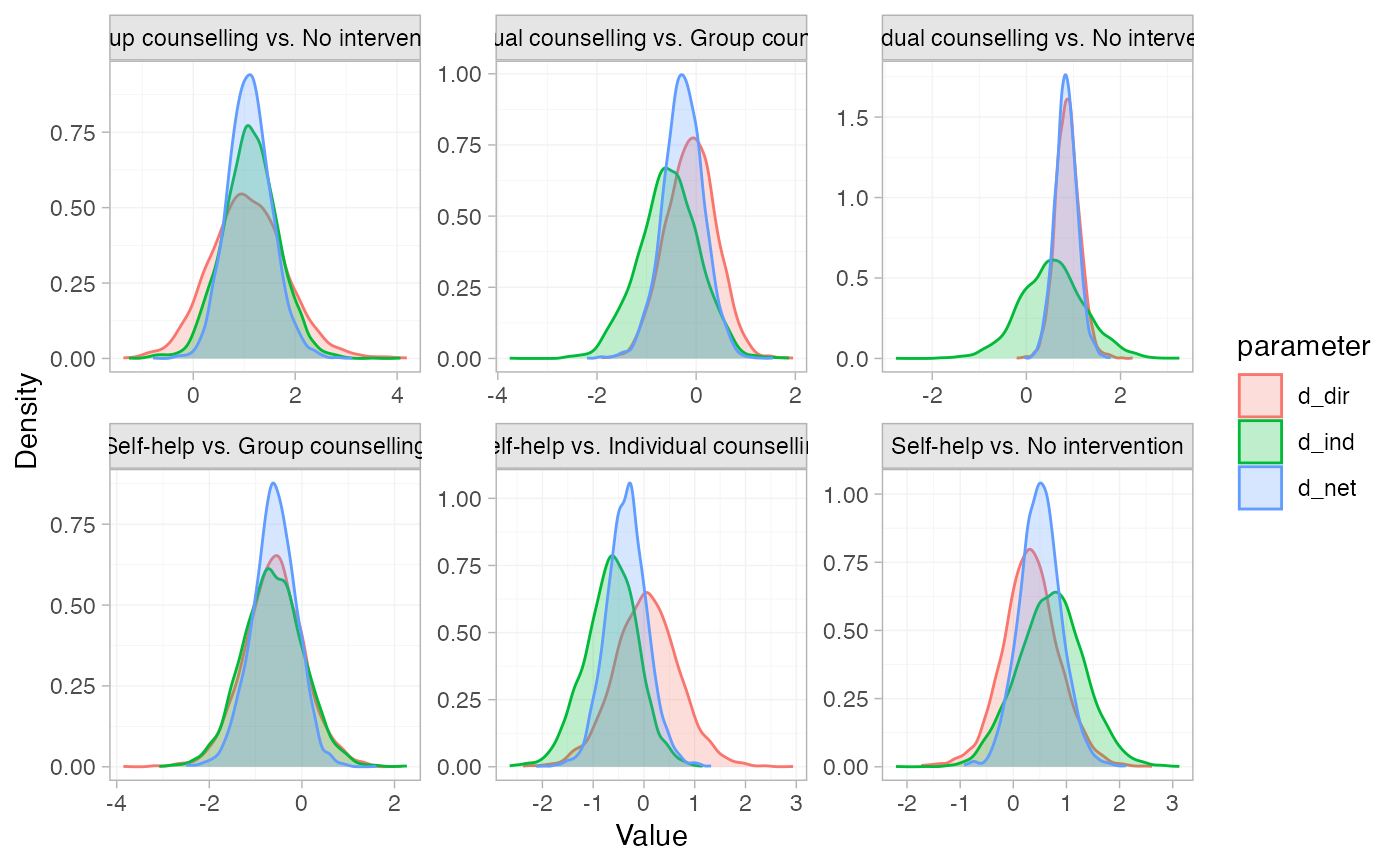
# Plot the node-splitting results
plot(smk_fit_RE_nodesplit)
 # }
# }