#> For execution on a local, multicore CPU with excess RAM we recommend calling
#> options(mc.cores = parallel::detectCores())
#>
#> Attaching package: 'multinma'
#> The following objects are masked from 'package:stats':
#>
#>     dgamma, pgamma, qgamma
This vignette describes the analysis of 22 trials comparing beta
blockers to control for preventing mortality after myocardial infarction
(Carlin 1992; Dias et al. 2011). The data are available in
this package as blocker:
head(blocker)
#>   studyn trtn         trtc  r   n
#> 1      1    1      Control  3  39
#> 2      1    2 Beta Blocker  3  38
#> 3      2    1      Control 14 116
#> 4      2    2 Beta Blocker  7 114
#> 5      3    1      Control 11  93
#> 6      3    2 Beta Blocker  5  69
Setting up the network
We begin by setting up the network - here just a pairwise
meta-analysis. We have arm-level count data giving the number of deaths
(r) out of the total (n) in each arm, so we
use the function set_agd_arm(). We set “Control” as the
reference treatment.
blocker_net <- set_agd_arm(blocker,
                           study = studyn,
                           trt = trtc,
                           r = r,
                           n = n,
                           trt_ref = "Control")
blocker_net
#> A network with 22 AgD studies (arm-based).
#>
#> ------------------------------------------------------- AgD studies (arm-based) ----
#>  Study Treatment arms
#>  1     2: Control | Beta Blocker
#>  2     2: Control | Beta Blocker
#>  3     2: Control | Beta Blocker
#>  4     2: Control | Beta Blocker
#>  5     2: Control | Beta Blocker
#>  6     2: Control | Beta Blocker
#>  7     2: Control | Beta Blocker
#>  8     2: Control | Beta Blocker
#>  9     2: Control | Beta Blocker
#>  10    2: Control | Beta Blocker
#>  ... plus 12 more studies
#>
#>  Outcome type: count
#> ------------------------------------------------------------------------------------
#> Total number of treatments: 2
#> Total number of studies: 22
#> Reference treatment is: Control
#> Network is connected
Meta-analysis models
We fit both fixed effect (FE) and random effects (RE) models.
Fixed effect meta-analysis
First, we fit a fixed effect model using the nma()
function with trt_effects = "fixed". We use \mathrm{N}(0, 100^2) prior distributions for
the treatment effects d_k and
study-specific intercepts \mu_j. We can
examine the range of parameter values implied by these prior
distributions with the summary() method:
summary(normal(scale = 100))
#> A Normal prior distribution: location = 0, scale = 100.
#> 50% of the prior density lies between -67.45 and 67.45.
#> 95% of the prior density lies between -196 and 196.
The model is fitted using the nma() function. By
default, this will use a Binomial likelihood and a logit link function,
auto-detected from the data.
blocker_fit_FE <- nma(blocker_net,
                   trt_effects = "fixed",
                   prior_intercept = normal(scale = 100),
                   prior_trt = normal(scale = 100))
Basic parameter summaries are given by the print()
method:
blocker_fit_FE
#> A fixed effects NMA with a binomial likelihood (logit link).
#> Inference for Stan model: binomial_1par.
#> 4 chains, each with iter=2000; warmup=1000; thin=1;
#> post-warmup draws per chain=1000, total post-warmup draws=4000.
#>
#>                     mean se_mean   sd     2.5%      25%      50%      75%    97.5% n_eff Rhat
#> d[Beta Blocker]    -0.26    0.00 0.05    -0.36    -0.30    -0.26    -0.23    -0.16  3693    1
#> lp__            -5960.39    0.09 3.48 -5968.17 -5962.42 -5960.09 -5957.94 -5954.57  1363    1
#>
#> Samples were drawn using NUTS(diag_e) at Fri Jun 26 12:35:32 2026.
#> For each parameter, n_eff is a crude measure of effective sample size,
#> and Rhat is the potential scale reduction factor on split chains (at
#> convergence, Rhat=1).
By default, summaries of the study-specific intercepts \mu_j are hidden, but could be examined by
changing the pars argument:
The prior and posterior distributions can be compared visually using
the plot_prior_posterior() function:
plot_prior_posterior(blocker_fit_FE, prior = "trt")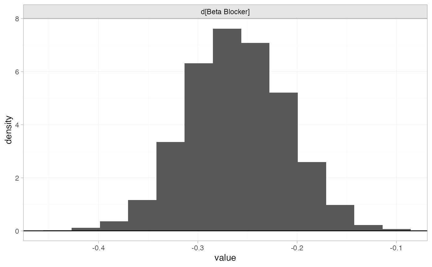
Random effects meta-analysis
We now fit a random effects model using the nma()
function with trt_effects = "random". Again, we use \mathrm{N}(0, 100^2) prior distributions for
the treatment effects d_k and
study-specific intercepts \mu_j, and we
additionally use a \textrm{half-N}(5^2)
prior for the heterogeneity standard deviation \tau. We can examine the range of parameter
values implied by these prior distributions with the
summary() method:
summary(normal(scale = 100))
#> A Normal prior distribution: location = 0, scale = 100.
#> 50% of the prior density lies between -67.45 and 67.45.
#> 95% of the prior density lies between -196 and 196.
summary(half_normal(scale = 5))
#> A half-Normal prior distribution: scale = 5.
#> 50% of the prior density lies between 0 and 3.37.
#> 95% of the prior density lies between 0 and 9.8.
Fitting the RE model
blocker_fit_RE <- nma(blocker_net,
                   trt_effects = "random",
                   prior_intercept = normal(scale = 100),
                   prior_trt = normal(scale = 100),
                   prior_het = half_normal(scale = 5))
Basic parameter summaries are given by the print()
method:
blocker_fit_RE
#> A random effects NMA with a binomial likelihood (logit link).
#> Inference for Stan model: binomial_1par.
#> 4 chains, each with iter=2000; warmup=1000; thin=1;
#> post-warmup draws per chain=1000, total post-warmup draws=4000.
#>
#>                     mean se_mean   sd     2.5%      25%      50%      75%    97.5% n_eff Rhat
#> d[Beta Blocker]    -0.25    0.00 0.06    -0.38    -0.29    -0.25    -0.21    -0.13  4174    1
#> lp__            -5970.70    0.17 5.66 -5982.57 -5974.43 -5970.52 -5966.81 -5960.34  1072    1
#> tau                 0.13    0.00 0.08     0.01     0.07     0.13     0.19     0.31   928    1
#>
#> Samples were drawn using NUTS(diag_e) at Fri Jun 26 12:35:35 2026.
#> For each parameter, n_eff is a crude measure of effective sample size,
#> and Rhat is the potential scale reduction factor on split chains (at
#> convergence, Rhat=1).
By default, summaries of the study-specific intercepts \mu_j and study-specific relative effects
\delta_{jk} are hidden, but could be
examined by changing the pars argument:
The prior and posterior distributions can be compared visually using
the plot_prior_posterior() function:
plot_prior_posterior(blocker_fit_RE, prior = c("trt", "het"))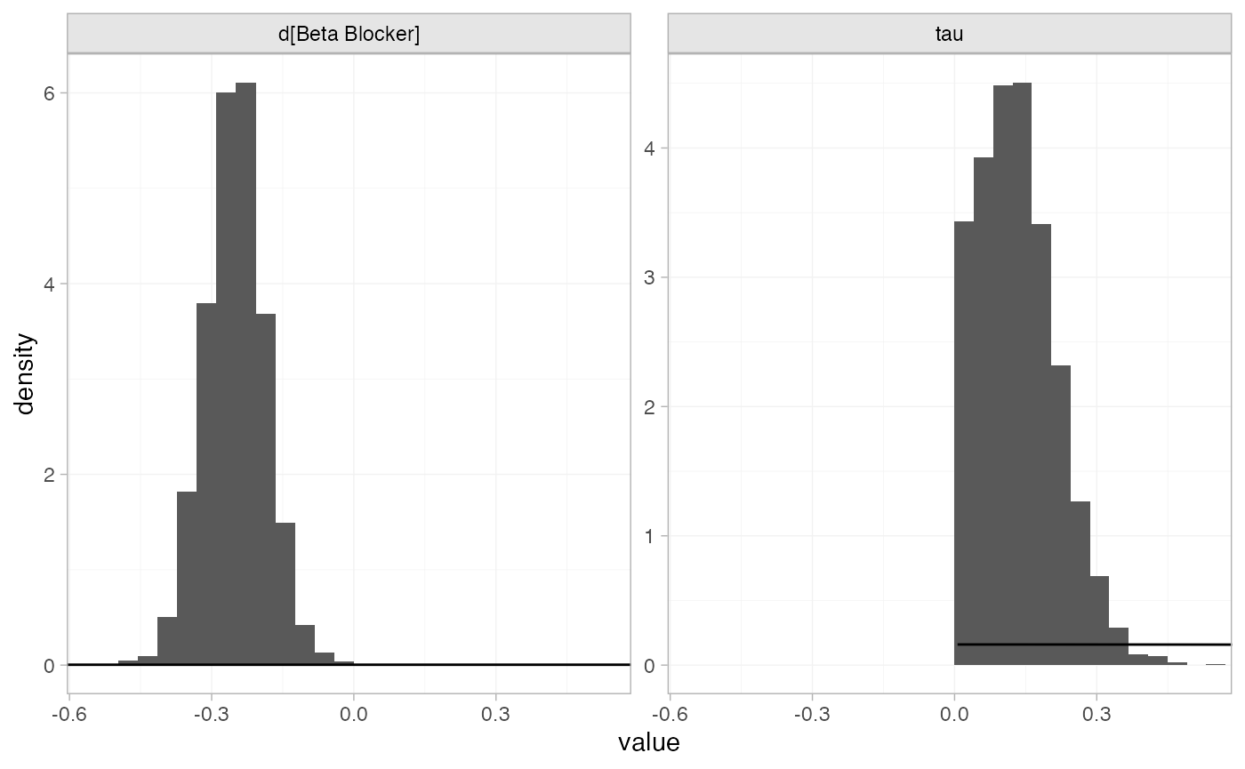
Model comparison
Model fit can be checked using the dic() function:
(dic_FE <- dic(blocker_fit_FE))
#> Residual deviance: 46.8 (on 44 data points)
#>                pD: 23.1
#>               DIC: 69.9
(dic_RE <- dic(blocker_fit_RE))
#> Residual deviance: 41.8 (on 44 data points)
#>                pD: 28.1
#>               DIC: 69.9
The residual deviance is lower under the RE model, which is to be expected as this model is more flexible. However, this comes with an increased effective number of parameters (note the increase in p_D). As a result, the DIC of both models is very similar and the FE model may be preferred for parsimony.
We can also examine the residual deviance contributions with the
corresponding plot() method.
plot(dic_FE)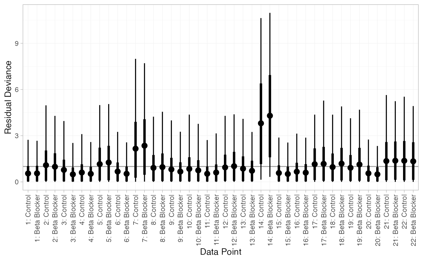
plot(dic_RE)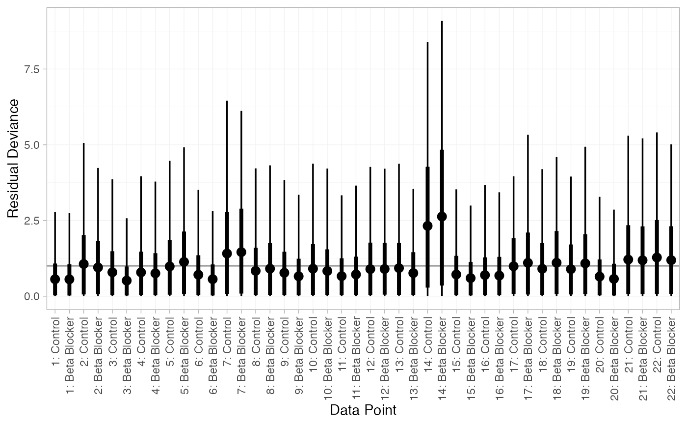
There are a number of points which are not very well fit by the FE model, having posterior mean residual deviance contributions greater than 1. Study 14 is a particularly poor fit under the FE model, but its residual deviance is reduced (although still high) under the RE model. The evidence should be given further careful examination, and consideration given to other issues such as the potential for effect-modifying covariates (Dias et al. 2011).
Leverage plots can also be produced with the plot()
method, with type = "leverage".
plot(dic_FE, type = "leverage") +
  # Add labels for points outside DIC=3
  geom_text(aes(label = parameter), data = ~subset(., dic > 3), vjust = -0.5)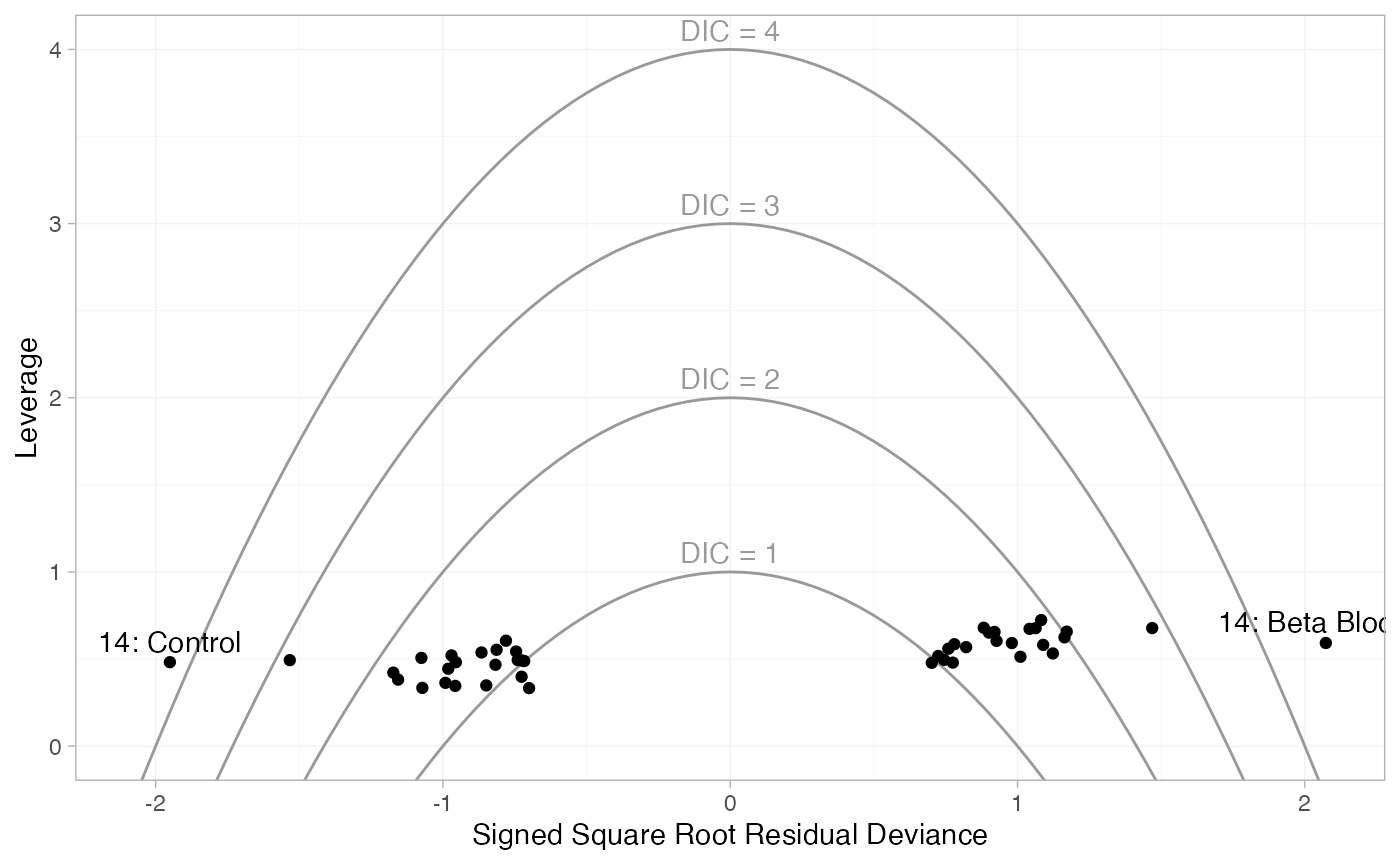
plot(dic_RE, type = "leverage") +
  # Add labels for points outside DIC=3
  geom_text(aes(label = parameter), data = ~subset(., dic > 3), vjust = -0.5)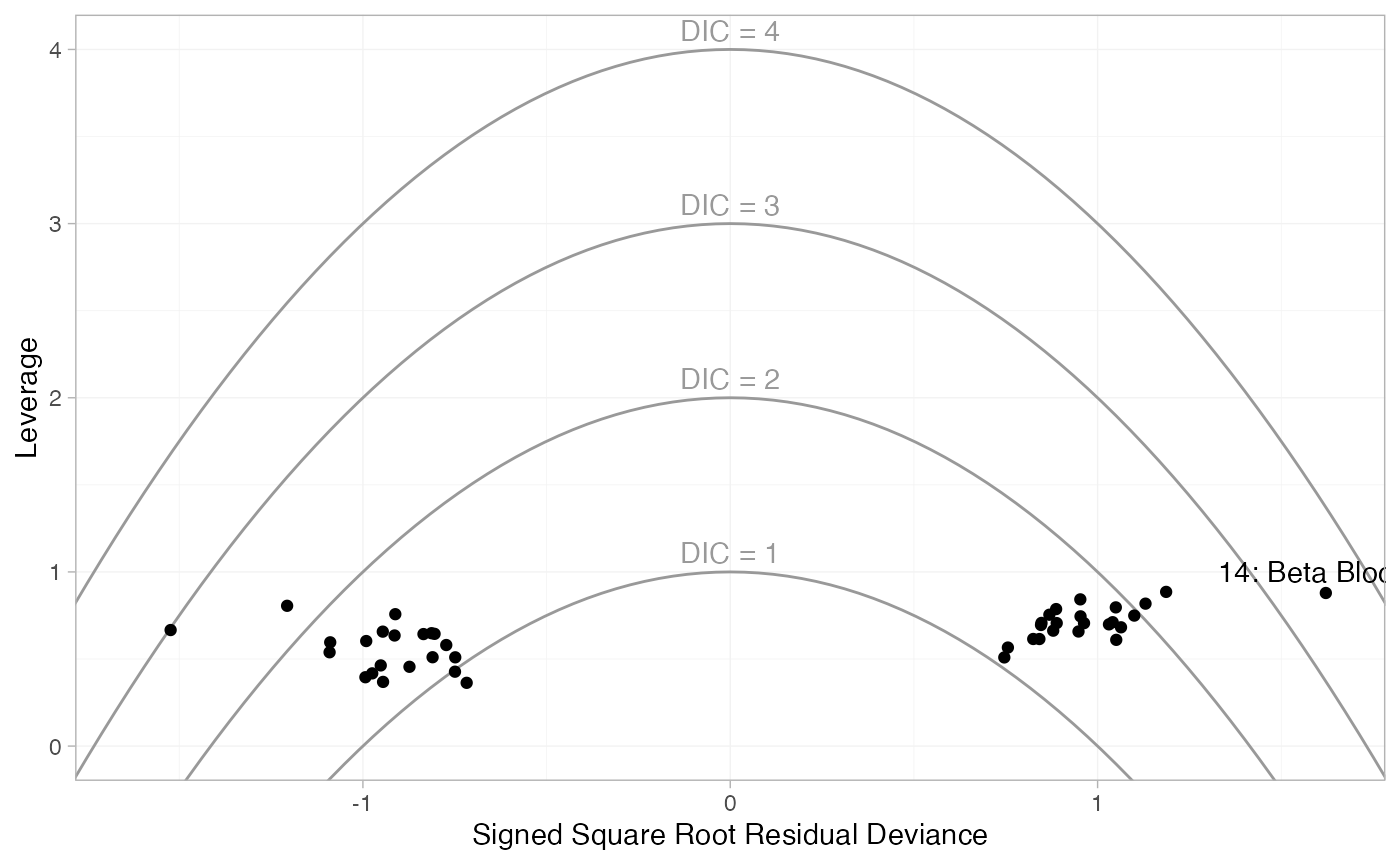
These plot the leverage for each data point (i.e. its contribution to
model complexity p_D) against the
square root of the residual deviance. The sign of the square root
residual deviance is given by sign of the difference between the
observed and model-predicted values, indicating whether each data point
is under- or over-estimated by the model. Contours are displayed which
indicate lines of constant contribution to the DIC. Points contributing
more than 3 to the DIC are generally considered to be contributing to
poor fit; here we have labelled these points using the
ggplot2 function geom_text(). As with the
residual deviance plots above, we again see that both arms of study 14
are fit poorly under the FE model, and their fit is improved (but still
poor) under the RE model.
Further results
Dias et al. (2011) produce absolute predictions of the
probability of mortality on beta blockers and control, assuming a Normal
distribution on the baseline logit-probability of mortality with mean
-2.2 and precision 3.3. We can replicate these results using the
predict() method. The baseline argument takes
a distr() distribution object, with which we specify the
corresponding Normal distribution. We set type = "response"
to produce predicted probabilities (type = "link" would
produce predicted log odds).
pred_FE <- predict(blocker_fit_FE,
                   baseline = distr(qnorm, mean = -2.2, sd = 3.3^-0.5),
                   type = "response")
pred_FE
#>                    mean   sd 2.5%  25%  50%  75% 97.5% Bulk_ESS Tail_ESS Rhat
#> pred[Control]      0.11 0.05 0.04 0.07 0.10 0.14  0.24     4073     3875    1
#> pred[Beta Blocker] 0.09 0.04 0.03 0.06 0.08 0.11  0.19     4086     3948    1
plot(pred_FE)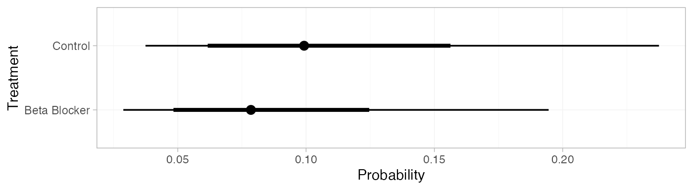
pred_RE <- predict(blocker_fit_RE,
                   baseline = distr(qnorm, mean = -2.2, sd = 3.3^-0.5),
                   type = "response")
pred_RE
#>                    mean   sd 2.5%  25%  50%  75% 97.5% Bulk_ESS Tail_ESS Rhat
#> pred[Control]      0.11 0.05 0.04 0.07 0.10 0.14  0.25     4384     3718    1
#> pred[Beta Blocker] 0.09 0.05 0.03 0.06 0.08 0.11  0.20     4373     3486    1
plot(pred_RE)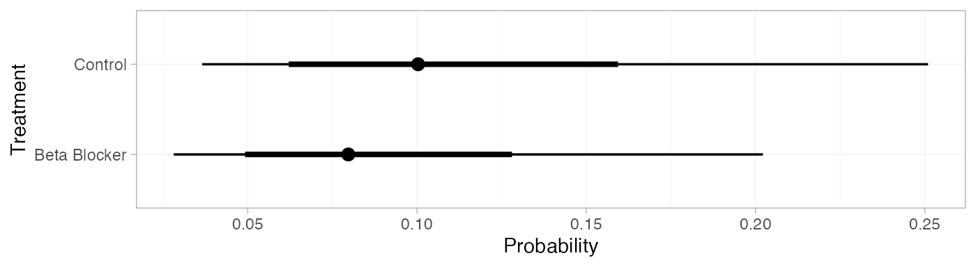
If instead of information on the baseline logit-probability of
mortality we have event counts, we can use these to construct a Beta
distribution for the baseline probability of mortality. For example, if
4 out of 36 individuals died on control treatment in the target
population of interest, the appropriate Beta distribution for the
probability would be \textrm{Beta}(4,
36-4). We can specify this Beta distribution for the baseline
response using the baseline_type = "reponse" argument (the
default is "link", used above for the baseline
logit-probability).
pred_FE_beta <- predict(blocker_fit_FE,
                        baseline = distr(qbeta, 4, 36-4),
                        baseline_type = "response",
                        type = "response")
pred_FE_beta
#>                    mean   sd 2.5%  25%  50%  75% 97.5% Bulk_ESS Tail_ESS Rhat
#> pred[Control]      0.11 0.05 0.03 0.07 0.10 0.14  0.23     3493     3846    1
#> pred[Beta Blocker] 0.09 0.04 0.02 0.06 0.08 0.11  0.19     3523     3885    1
plot(pred_FE_beta)
pred_RE_beta <- predict(blocker_fit_RE,
                        baseline = distr(qbeta, 4, 36-4),
                        baseline_type = "response",
                        type = "response")
pred_RE_beta
#>                    mean   sd 2.5%  25%  50%  75% 97.5% Bulk_ESS Tail_ESS Rhat
#> pred[Control]      0.11 0.05 0.03 0.07 0.10 0.14  0.23     3990     3890    1
#> pred[Beta Blocker] 0.09 0.04 0.03 0.06 0.08 0.11  0.19     4017     3918    1
plot(pred_RE_beta)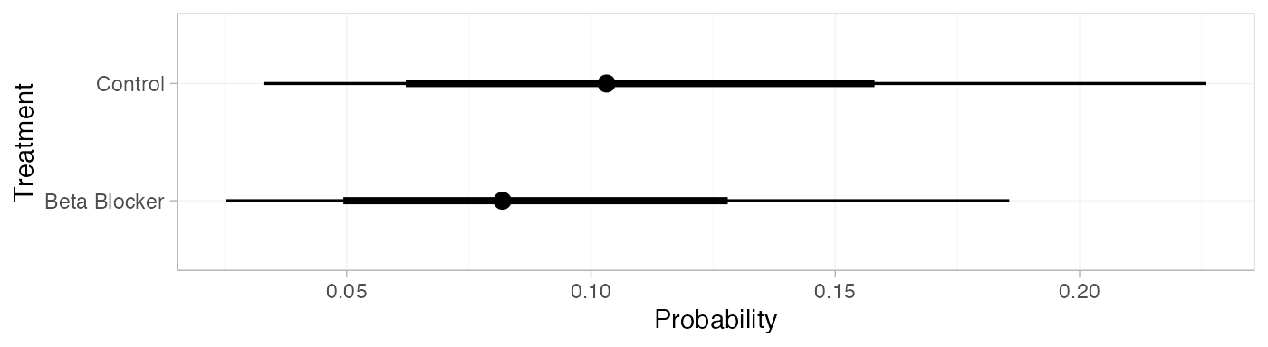
Notice that these results are nearly equivalent to those calculated above using the Normal distribution for the baseline logit-probability, since these event counts correspond to approximately the same distribution on the logit-probability.