Produce summary plots of node-splitting models
Arguments
- x
A
nodesplit_summaryobject.- ...
Additional arguments passed on to the underlying
ggdistplot stat, see Details.- pars
Character vector specifying the parameters to include in the plot, choices include
"d"for the direct, indirect, and network estimates of relative effects,"omega"for the inconsistency factor, and"tau"for heterogeneity standard deviation in random effects models. Default is"d".- stat
Character string specifying the
ggdistplot stat to use. The default"dens_overlay"is a special case, producing an overlaid density plot.- orientation
Whether the
ggdistgeom is drawn horizontally ("horizontal") or vertically ("vertical"), default"horizontal".- ref_line
Numeric vector of positions for reference lines, by default no reference lines are drawn.
Details
Plotting is handled by ggplot2 and
the stats and geoms provided in the ggdist
package. As a result, the output is very flexible. Any plotting stats
provided by ggdist may be used, via the argument stat. The default
"dens_overlay" is a special exception, which uses
ggplot2::geom_density(), to plot
overlaid densities. Additional arguments in ... are passed to the
ggdist stat, to customise the output.
Alternative stats can be specified to produce different summaries. For
example, specify stat = "[half]eye" to produce (half) eye plots, or stat = "pointinterval" to produce point estimates and credible intervals.
A full list of options and examples is found in the ggdist vignette
vignette("slabinterval", package = "ggdist").
A ggplot object is returned which can be further modified through the
usual ggplot2 functions to add further
aesthetics, geoms, themes, etc.
Examples
# \donttest{
# Run smoking node-splitting example if not already available
if (!exists("smk_fit_RE_nodesplit")) example("example_smk_nodesplit", run.donttest = TRUE)
# }
# \donttest{
# Summarise the node-splitting results
(smk_nodesplit_summary <- summary(smk_fit_RE_nodesplit))
#> Node-splitting models fitted for 6 comparisons.
#>
#> ------------------------------ Node-split Group counselling vs. No intervention ----
#>
#> mean sd 2.5% 25% 50% 75% 97.5% Bulk_ESS Tail_ESS Rhat
#> d_net 1.11 0.44 0.26 0.83 1.10 1.39 1.99 1927 2107 1
#> d_dir 1.05 0.73 -0.36 0.57 1.03 1.50 2.56 3785 3043 1
#> d_ind 1.15 0.54 0.10 0.80 1.14 1.51 2.27 1895 2285 1
#> omega -0.11 0.88 -1.89 -0.69 -0.10 0.46 1.66 2666 2760 1
#> tau 0.86 0.20 0.55 0.72 0.83 0.97 1.35 1430 2206 1
#> tau_consistency 0.84 0.18 0.55 0.71 0.81 0.94 1.27 1610 2124 1
#>
#> Residual deviance: 54.4 (on 50 data points)
#> pD: 44.5
#> DIC: 99
#>
#> Bayesian p-value: 0.9
#>
#> ------------------------- Node-split Individual counselling vs. No intervention ----
#>
#> mean sd 2.5% 25% 50% 75% 97.5% Bulk_ESS Tail_ESS Rhat
#> d_net 0.85 0.24 0.41 0.69 0.84 1.00 1.35 1085 1736 1.01
#> d_dir 0.89 0.26 0.41 0.71 0.87 1.05 1.42 1615 2324 1.00
#> d_ind 0.58 0.67 -0.73 0.14 0.58 1.00 1.92 1805 1953 1.00
#> omega 0.31 0.70 -1.08 -0.15 0.30 0.75 1.73 1846 2206 1.00
#> tau 0.86 0.19 0.55 0.73 0.84 0.96 1.29 1516 2327 1.00
#> tau_consistency 0.84 0.18 0.55 0.71 0.81 0.94 1.27 1610 2124 1.00
#>
#> Residual deviance: 54.3 (on 50 data points)
#> pD: 44.3
#> DIC: 98.6
#>
#> Bayesian p-value: 0.66
#>
#> -------------------------------------- Node-split Self-help vs. No intervention ----
#>
#> mean sd 2.5% 25% 50% 75% 97.5% Bulk_ESS Tail_ESS Rhat
#> d_net 0.50 0.41 -0.28 0.24 0.51 0.77 1.31 2020 2280 1
#> d_dir 0.34 0.54 -0.74 0.00 0.34 0.69 1.41 3322 2728 1
#> d_ind 0.70 0.62 -0.49 0.28 0.68 1.10 1.96 1835 2357 1
#> omega -0.36 0.82 -2.02 -0.89 -0.34 0.18 1.21 2099 2545 1
#> tau 0.87 0.20 0.55 0.73 0.84 0.98 1.31 1085 1943 1
#> tau_consistency 0.84 0.18 0.55 0.71 0.81 0.94 1.27 1610 2124 1
#>
#> Residual deviance: 53.7 (on 50 data points)
#> pD: 44.2
#> DIC: 97.9
#>
#> Bayesian p-value: 0.67
#>
#> ----------------------- Node-split Individual counselling vs. Group counselling ----
#>
#> mean sd 2.5% 25% 50% 75% 97.5% Bulk_ESS Tail_ESS Rhat
#> d_net -0.26 0.41 -1.08 -0.52 -0.25 0.01 0.52 2847 2606 1
#> d_dir -0.11 0.48 -1.11 -0.41 -0.11 0.21 0.80 4340 2898 1
#> d_ind -0.55 0.63 -1.82 -0.96 -0.54 -0.14 0.63 1558 2069 1
#> omega 0.44 0.70 -0.96 -0.01 0.45 0.87 1.82 1607 1789 1
#> tau 0.87 0.19 0.56 0.73 0.84 0.97 1.33 1225 1989 1
#> tau_consistency 0.84 0.18 0.55 0.71 0.81 0.94 1.27 1610 2124 1
#>
#> Residual deviance: 53.8 (on 50 data points)
#> pD: 44.1
#> DIC: 97.8
#>
#> Bayesian p-value: 0.51
#>
#> ------------------------------------ Node-split Self-help vs. Group counselling ----
#>
#> mean sd 2.5% 25% 50% 75% 97.5% Bulk_ESS Tail_ESS Rhat
#> d_net -0.61 0.49 -1.61 -0.91 -0.60 -0.30 0.33 3000 2761 1
#> d_dir -0.61 0.66 -1.90 -1.04 -0.62 -0.20 0.75 3872 2823 1
#> d_ind -0.61 0.67 -1.96 -1.04 -0.60 -0.18 0.76 2028 2389 1
#> omega -0.01 0.89 -1.69 -0.59 -0.02 0.53 1.92 2125 2557 1
#> tau 0.87 0.20 0.56 0.73 0.85 0.98 1.33 1184 1964 1
#> tau_consistency 0.84 0.18 0.55 0.71 0.81 0.94 1.27 1610 2124 1
#>
#> Residual deviance: 54.1 (on 50 data points)
#> pD: 44.2
#> DIC: 98.3
#>
#> Bayesian p-value: 0.99
#>
#> ------------------------------- Node-split Self-help vs. Individual counselling ----
#>
#> mean sd 2.5% 25% 50% 75% 97.5% Bulk_ESS Tail_ESS Rhat
#> d_net -0.35 0.42 -1.20 -0.62 -0.34 -0.07 0.47 2437 2317 1
#> d_dir 0.06 0.64 -1.20 -0.36 0.07 0.48 1.33 2697 2632 1
#> d_ind -0.57 0.51 -1.57 -0.90 -0.57 -0.25 0.47 1886 2498 1
#> omega 0.63 0.80 -0.99 0.11 0.64 1.15 2.16 1929 2112 1
#> tau 0.85 0.19 0.55 0.72 0.83 0.96 1.29 1168 1591 1
#> tau_consistency 0.84 0.18 0.55 0.71 0.81 0.94 1.27 1610 2124 1
#>
#> Residual deviance: 53.8 (on 50 data points)
#> pD: 44.1
#> DIC: 98
#>
#> Bayesian p-value: 0.41
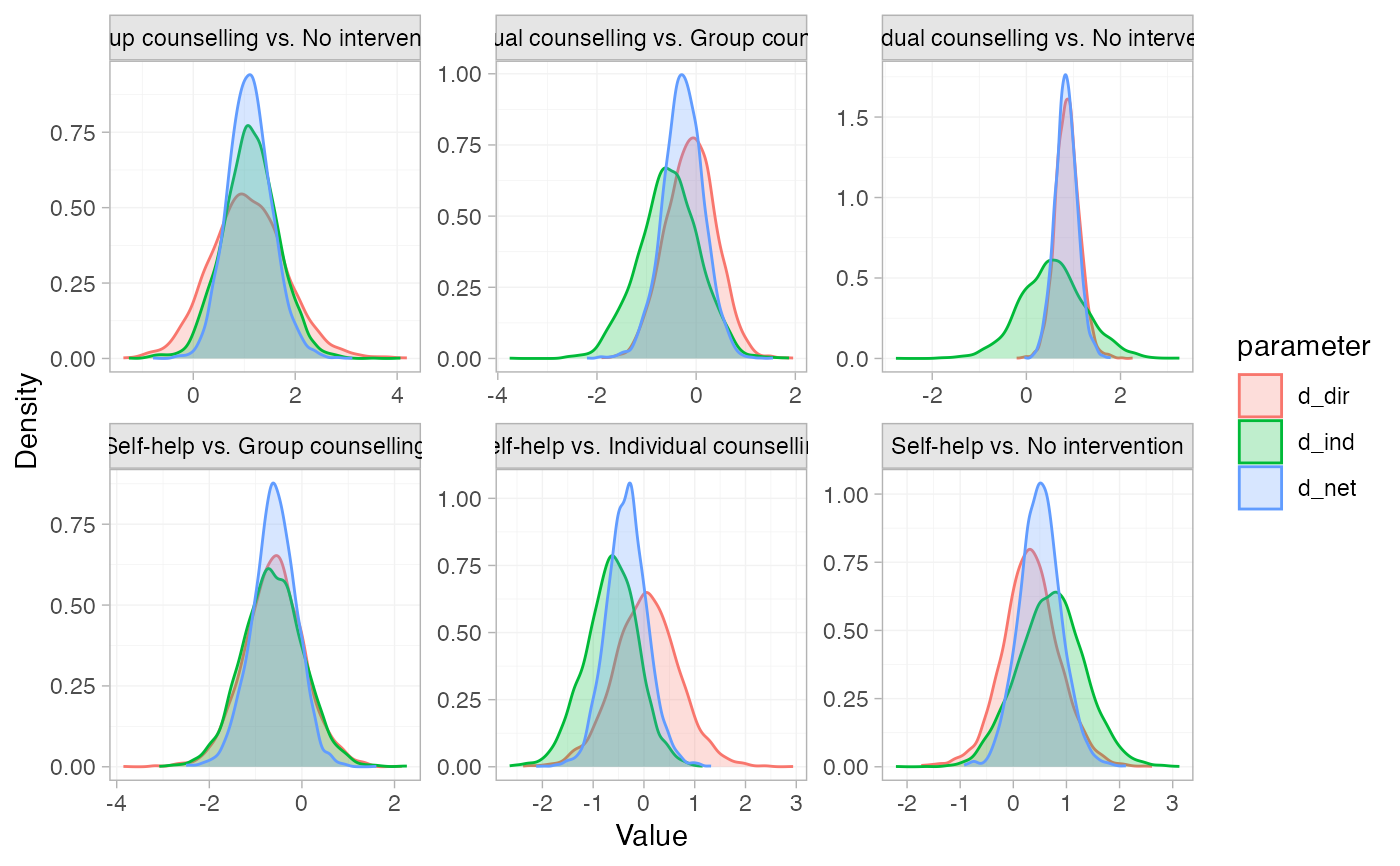
# Plot the node-splitting results
plot(smk_nodesplit_summary)
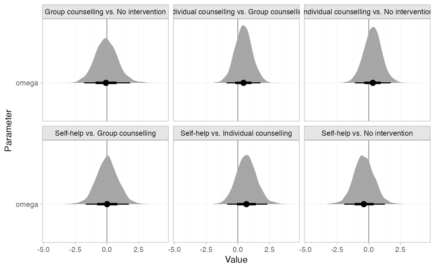
 # Plot the inconsistency factors instead, change the plot stat to half-eye,
# and add a reference line at 0
plot(smk_nodesplit_summary, pars = "omega", stat = "halfeye", ref_line = 0)
# Plot the inconsistency factors instead, change the plot stat to half-eye,
# and add a reference line at 0
plot(smk_nodesplit_summary, pars = "omega", stat = "halfeye", ref_line = 0)
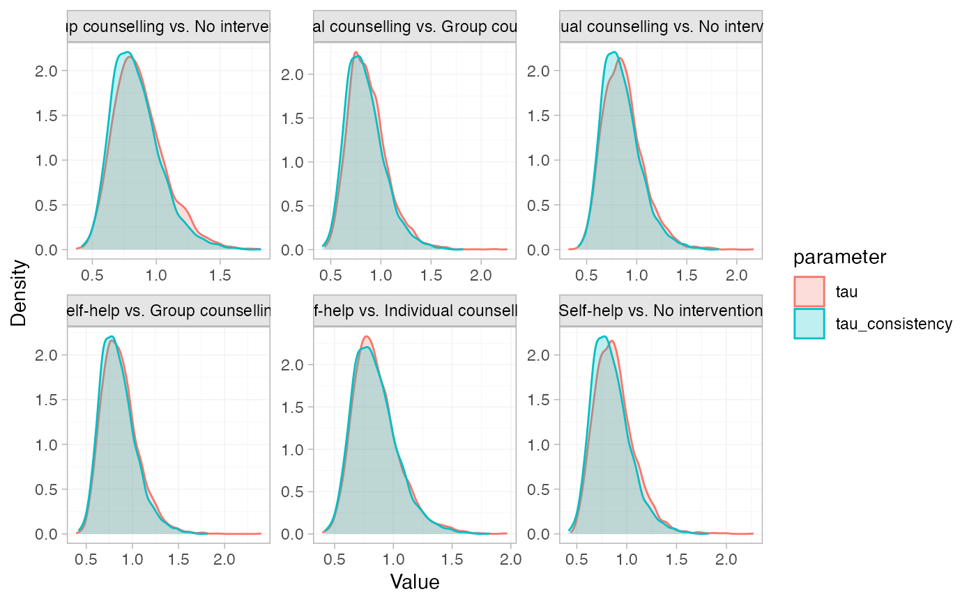
 # Plot a comparison of the heterogeneity under the node-split models vs.
# the consistency model
plot(smk_nodesplit_summary, pars = "tau")
# Plot a comparison of the heterogeneity under the node-split models vs.
# the consistency model
plot(smk_nodesplit_summary, pars = "tau")
 # }
# }