Example: Parkinson's disease

library(multinma)
options(mc.cores = parallel::detectCores())

#> For execution on a local, multicore CPU with excess RAM we recommend calling
#> options(mc.cores = parallel::detectCores())
#> 
#> Attaching package: 'multinma'
#> The following objects are masked from 'package:stats':
#> 
#>     dgamma, pgamma, qgamma

This vignette describes the analysis of data on the mean off-time reduction in patients given dopamine agonists as adjunct therapy in Parkinson’s disease, in a network of 7 trials of 4 active drugs plus placebo (Dias et al. 2011). The data are available in this package as parkinsons:

head(parkinsons)
#>   studyn trtn     y    se   n  diff se_diff
#> 1      1    1 -1.22 0.504  54    NA   0.504
#> 2      1    3 -1.53 0.439  95 -0.31   0.668
#> 3      2    1 -0.70 0.282 172    NA   0.282
#> 4      2    2 -2.40 0.258 173 -1.70   0.382
#> 5      3    1 -0.30 0.505  76    NA   0.505
#> 6      3    2 -2.60 0.510  71 -2.30   0.718

We consider analysing these data in three separate ways:

1. Using arm-based data (means y and corresponding standard errors se);
2. Using contrast-based data (mean differences diff and corresponding standard errors se_diff);
3. A combination of the two, where some studies contribute arm-based data, and other contribute contrast-based data.

Note: In this case, with Normal likelihoods for both arms and contrasts, we will see that the three analyses give identical results. In general, unless the arm-based likelihood is Normal, results from a model using a contrast-based likelihood will not exactly match those from a model using an arm-based likelihood, since the contrast-based Normal likelihood is only an approximation. Similarity of results depends on the suitability of the Normal approximation, which may not always be appropriate - e.g. with a small number of events or small sample size for a binary outcome. The use of an arm-based likelihood (sometimes called an “exact” likelihood) is therefore preferable where possible in general.

Analysis of arm-based data

We begin with an analysis of the arm-based data - means and standard errors.

Setting up the network

We have arm-level continuous data giving the mean off-time reduction (y) and standard error (se) in each arm. We use the function set_agd_arm() to set up the network.

arm_net <- set_agd_arm(parkinsons, 
                      study = studyn,
                      trt = trtn,
                      y = y, 
                      se = se,
                      sample_size = n)
arm_net
#> A network with 7 AgD studies (arm-based).
#> 
#> ------------------------------------------------------- AgD studies (arm-based) ---- 
#>  Study Treatment arms
#>  1     2: 1 | 3      
#>  2     2: 1 | 2      
#>  3     3: 4 | 1 | 2  
#>  4     2: 4 | 3      
#>  5     2: 4 | 3      
#>  6     2: 4 | 5      
#>  7     2: 4 | 5      
#> 
#>  Outcome type: continuous
#> ------------------------------------------------------------------------------------
#> Total number of treatments: 5
#> Total number of studies: 7
#> Reference treatment is: 4
#> Network is connected

We let treatment 4 be set by default as the network reference treatment, since this results in considerably improved sampling efficiency over choosing treatment 1 as the network reference. The sample_size argument is optional, but enables the nodes to be weighted by sample size in the network plot.

Plot the network structure.

plot(arm_net, weight_edges = TRUE, weight_nodes = TRUE)

Meta-analysis models

We fit both fixed effect (FE) and random effects (RE) models.

Fixed effect meta-analysis

First, we fit a fixed effect model using the nma() function with trt_effects = "fixed". We use $\mathrm{N}(0, 100^2)$ prior distributions for the treatment effects $d_k$ and study-specific intercepts $\mu_j$. We can examine the range of parameter values implied by these prior distributions with the summary() method:

summary(normal(scale = 100))
#> A Normal prior distribution: location = 0, scale = 100.
#> 50% of the prior density lies between -67.45 and 67.45.
#> 95% of the prior density lies between -196 and 196.

The model is fitted using the nma() function.

arm_fit_FE <- nma(arm_net, 
                  trt_effects = "fixed",
                  prior_intercept = normal(scale = 100),
                  prior_trt = normal(scale = 10))
#> Note: Setting "4" as the network reference treatment.

Basic parameter summaries are given by the print() method:

arm_fit_FE
#> A fixed effects NMA with a normal likelihood (identity link).
#> Inference for Stan model: normal.
#> 4 chains, each with iter=2000; warmup=1000; thin=1; 
#> post-warmup draws per chain=1000, total post-warmup draws=4000.
#> 
#>       mean se_mean   sd   2.5%   25%   50%   75% 97.5% n_eff Rhat
#> d[1]  0.54    0.01 0.47  -0.38  0.23  0.55  0.86  1.47  1503    1
#> d[2] -1.26    0.01 0.52  -2.29 -1.61 -1.26 -0.91 -0.26  1555    1
#> d[3]  0.05    0.01 0.33  -0.60 -0.18  0.04  0.27  0.68  1965    1
#> d[5] -0.30    0.00 0.22  -0.73 -0.45 -0.30 -0.15  0.12  3127    1
#> lp__ -6.76    0.06 2.41 -12.44 -8.12 -6.42 -5.02 -3.12  1724    1
#> 
#> Samples were drawn using NUTS(diag_e) at Tue Sep 24 09:07:43 2024.
#> For each parameter, n_eff is a crude measure of effective sample size,
#> and Rhat is the potential scale reduction factor on split chains (at 
#> convergence, Rhat=1).

By default, summaries of the study-specific intercepts $\mu_j$ are hidden, but could be examined by changing the pars argument:

# Not run
print(arm_fit_FE, pars = c("d", "mu"))

The prior and posterior distributions can be compared visually using the plot_prior_posterior() function:

plot_prior_posterior(arm_fit_FE)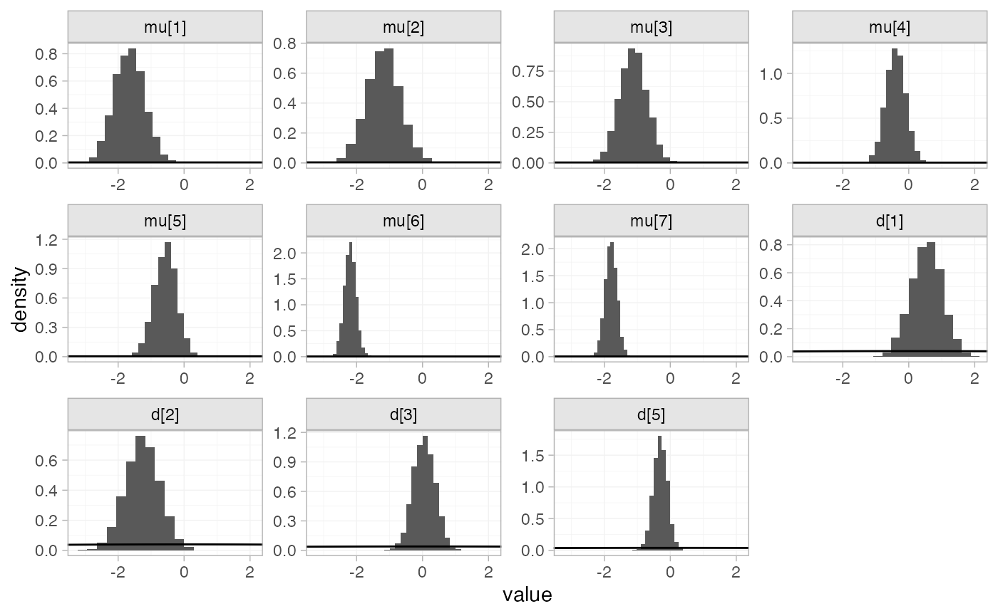

Random effects meta-analysis

We now fit a random effects model using the nma() function with trt_effects = "random". Again, we use $\mathrm{N}(0, 100^2)$ prior distributions for the treatment effects $d_k$ and study-specific intercepts $\mu_j$, and we additionally use a $\textrm{half-N}(5^2)$ prior for the heterogeneity standard deviation $\tau$. We can examine the range of parameter values implied by these prior distributions with the summary() method:

summary(normal(scale = 100))
#> A Normal prior distribution: location = 0, scale = 100.
#> 50% of the prior density lies between -67.45 and 67.45.
#> 95% of the prior density lies between -196 and 196.
summary(half_normal(scale = 5))
#> A half-Normal prior distribution: location = 0, scale = 5.
#> 50% of the prior density lies between 0 and 3.37.
#> 95% of the prior density lies between 0 and 9.8.

Fitting the RE model

arm_fit_RE <- nma(arm_net, 
                  seed = 379394727,
                  trt_effects = "random",
                  prior_intercept = normal(scale = 100),
                  prior_trt = normal(scale = 100),
                  prior_het = half_normal(scale = 5),
                  adapt_delta = 0.99)
#> Note: Setting "4" as the network reference treatment.
#> Warning: There were 3 divergent transitions after warmup. See
#> https://mc-stan.org/misc/warnings.html#divergent-transitions-after-warmup
#> to find out why this is a problem and how to eliminate them.
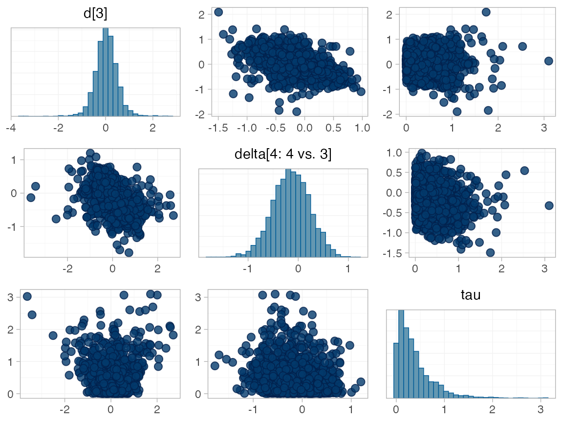
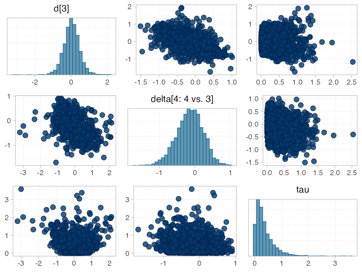
#> Warning: Examine the pairs() plot to diagnose sampling problems

We do see a small number of divergent transition errors, which cannot simply be removed by increasing the value of the adapt_delta argument (by default set to 0.95 for RE models). To diagnose, we use the pairs() method to investigate where in the posterior distribution these divergences are happening (indicated by red crosses):

pairs(arm_fit_RE, pars = c("mu[4]", "d[3]", "delta[4: 3]", "tau"))

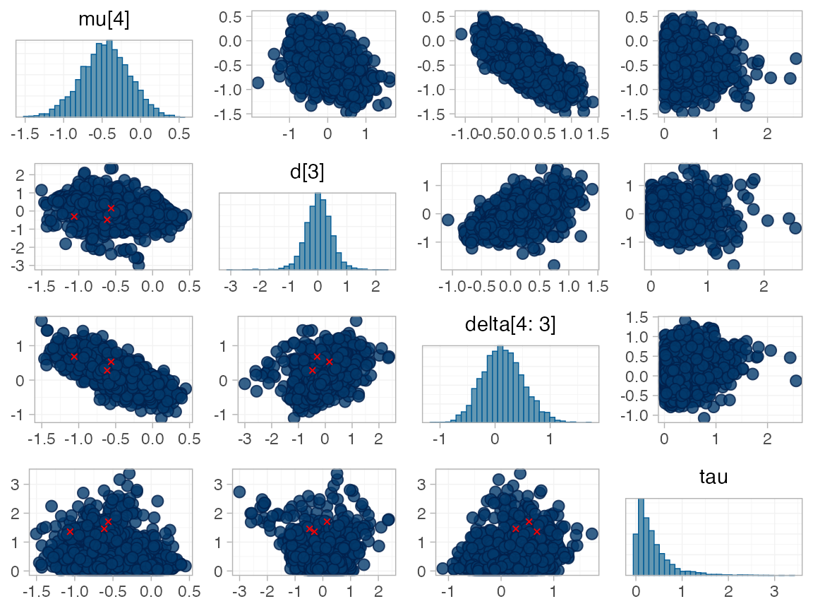
The divergent transitions occur in the upper tail of the heterogeneity standard deviation. In this case, with only a small number of studies, there is not very much information to estimate the heterogeneity standard deviation and the prior distribution may be too heavy-tailed. We could consider a more informative prior distribution for the heterogeneity variance to aid estimation.

Basic parameter summaries are given by the print() method:

arm_fit_RE
#> A random effects NMA with a normal likelihood (identity link).
#> Inference for Stan model: normal.
#> 4 chains, each with iter=2000; warmup=1000; thin=1; 
#> post-warmup draws per chain=1000, total post-warmup draws=4000.
#> 
#>        mean se_mean   sd   2.5%    25%    50%    75% 97.5% n_eff Rhat
#> d[1]   0.53    0.01 0.61  -0.65   0.15   0.55   0.91  1.69  1935    1
#> d[2]  -1.33    0.02 0.71  -2.72  -1.75  -1.31  -0.88 -0.05  1448    1
#> d[3]   0.02    0.01 0.47  -0.90  -0.25   0.03   0.31  0.91  1999    1
#> d[5]  -0.29    0.01 0.41  -1.09  -0.49  -0.29  -0.10  0.54  2340    1
#> lp__ -13.00    0.10 3.53 -20.90 -15.16 -12.71 -10.46 -7.04  1160    1
#> tau    0.37    0.02 0.39   0.01   0.11   0.26   0.49  1.46   516    1
#> 
#> Samples were drawn using NUTS(diag_e) at Tue Sep 24 09:07:47 2024.
#> For each parameter, n_eff is a crude measure of effective sample size,
#> and Rhat is the potential scale reduction factor on split chains (at 
#> convergence, Rhat=1).

By default, summaries of the study-specific intercepts $\mu_j$ and study-specific relative effects $\delta_{jk}$ are hidden, but could be examined by changing the pars argument:

# Not run
print(arm_fit_RE, pars = c("d", "mu", "delta"))

The prior and posterior distributions can be compared visually using the plot_prior_posterior() function:

plot_prior_posterior(arm_fit_RE)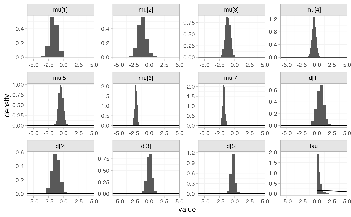

Model comparison

Model fit can be checked using the dic() function:

(arm_dic_FE <- dic(arm_fit_FE))
#> Residual deviance: 13.5 (on 15 data points)
#>                pD: 11.2
#>               DIC: 24.7

(arm_dic_RE <- dic(arm_fit_RE))
#> Residual deviance: 13.7 (on 15 data points)
#>                pD: 12.4
#>               DIC: 26.1

Both models fit the data well, having posterior mean residual deviance close to the number of data points. The DIC is similar between models, so we choose the FE model based on parsimony.

We can also examine the residual deviance contributions with the corresponding plot() method.

plot(arm_dic_FE)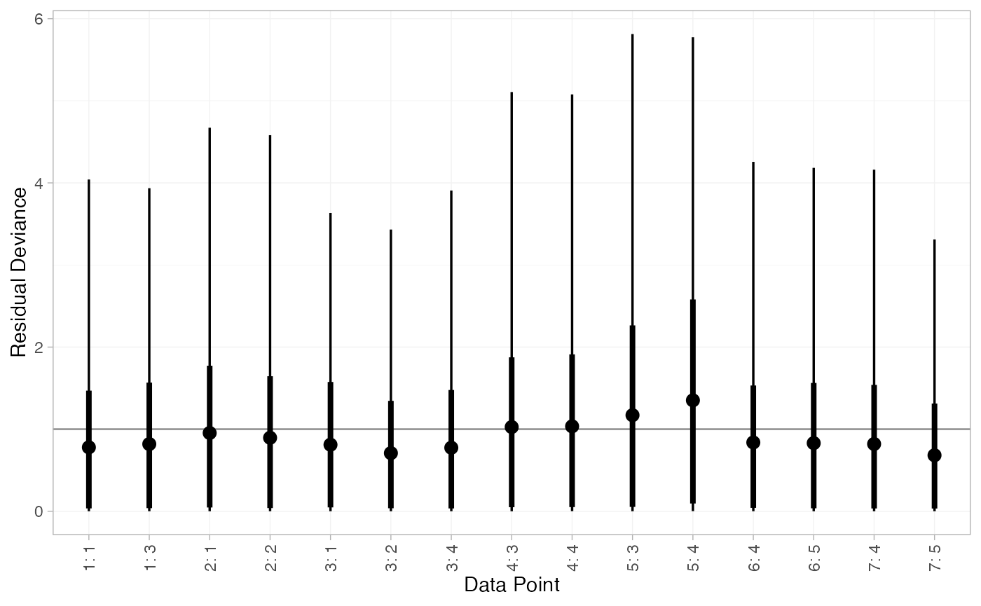

plot(arm_dic_RE)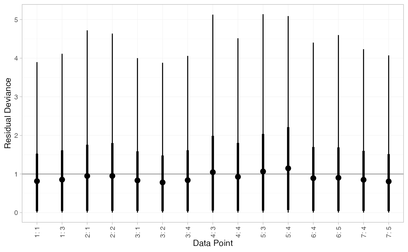

Further results

For comparison with Dias et al. (2011), we can produce relative effects against placebo using the relative_effects() function with trt_ref = 1:

(arm_releff_FE <- relative_effects(arm_fit_FE, trt_ref = 1))
#>       mean   sd  2.5%   25%   50%   75% 97.5% Bulk_ESS Tail_ESS Rhat
#> d[4] -0.54 0.47 -1.47 -0.86 -0.55 -0.23  0.38     1520     2166    1
#> d[2] -1.81 0.34 -2.46 -2.05 -1.81 -1.57 -1.13     5565     3253    1
#> d[3] -0.50 0.49 -1.43 -0.82 -0.50 -0.17  0.46     2474     2878    1
#> d[5] -0.84 0.52 -1.85 -1.19 -0.85 -0.50  0.17     1747     2429    1
plot(arm_releff_FE, ref_line = 0)

(arm_releff_RE <- relative_effects(arm_fit_RE, trt_ref = 1))
#>       mean   sd  2.5%   25%   50%   75% 97.5% Bulk_ESS Tail_ESS Rhat
#> d[4] -0.53 0.61 -1.69 -0.91 -0.55 -0.15  0.65     1998     1640    1
#> d[2] -1.86 0.54 -2.97 -2.14 -1.84 -1.55 -0.87     4450     1638    1
#> d[3] -0.50 0.64 -1.74 -0.88 -0.50 -0.12  0.72     3033     2509    1
#> d[5] -0.82 0.72 -2.19 -1.25 -0.84 -0.39  0.58     2075     1955    1
plot(arm_releff_RE, ref_line = 0)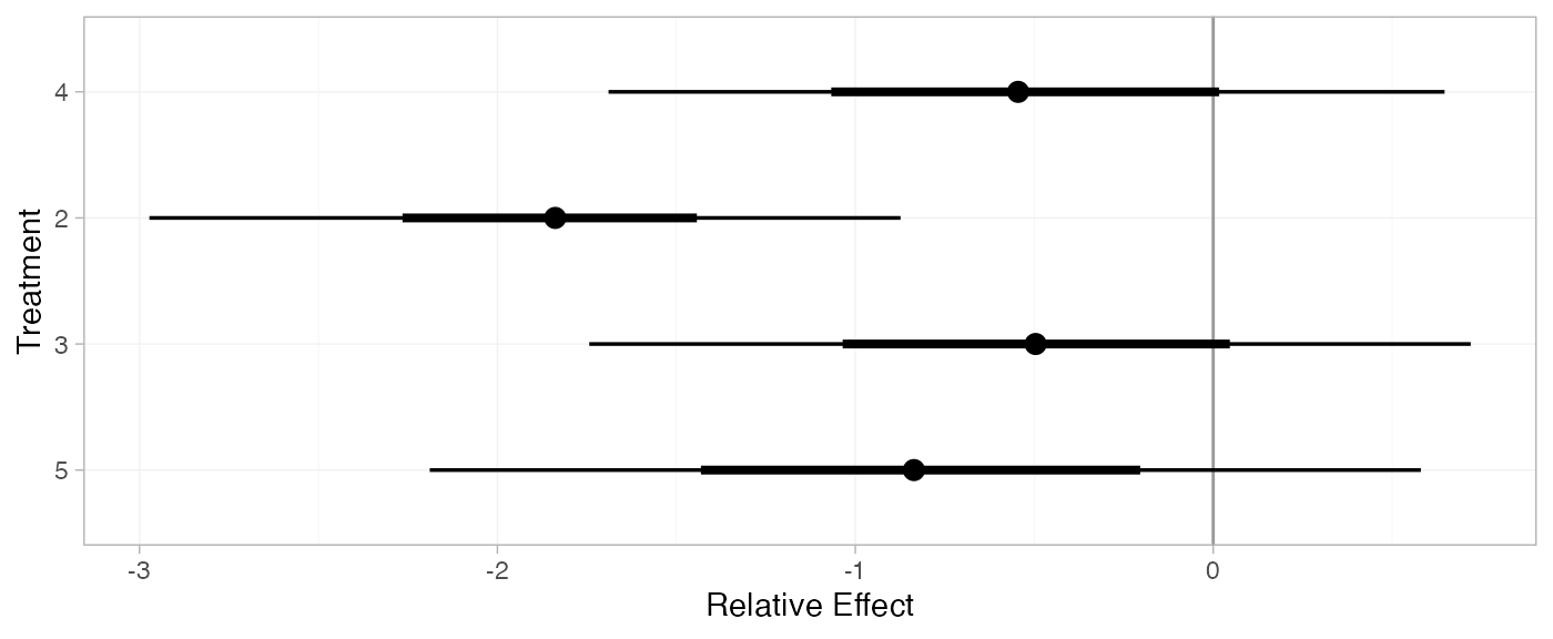

Following Dias et al. (2011), we produce absolute predictions of the mean off-time reduction on each treatment assuming a Normal distribution for the outcomes on treatment 1 (placebo) with mean $-0.73$ and precision $21$. We use the predict() method, where the baseline argument takes a distr() distribution object with which we specify the corresponding Normal distribution, and we specify baseline_trt = 1 to indicate that the baseline distribution corresponds to treatment 1. (Strictly speaking, type = "response" is unnecessary here, since the identity link function was used.)

arm_pred_FE <- predict(arm_fit_FE, 
                       baseline = distr(qnorm, mean = -0.73, sd = 21^-0.5),
                       type = "response",
                       baseline_trt = 1)
arm_pred_FE
#>          mean   sd  2.5%   25%   50%   75% 97.5% Bulk_ESS Tail_ESS Rhat
#> pred[4] -1.27 0.53 -2.29 -1.62 -1.28 -0.91 -0.24     1701     2585    1
#> pred[1] -0.73 0.22 -1.16 -0.88 -0.73 -0.58 -0.29     3910     3936    1
#> pred[2] -2.53 0.41 -3.33 -2.81 -2.53 -2.26 -1.74     5361     3716    1
#> pred[3] -1.22 0.54 -2.27 -1.59 -1.22 -0.86 -0.17     2650     3202    1
#> pred[5] -1.57 0.57 -2.68 -1.96 -1.58 -1.18 -0.44     1935     2716    1
plot(arm_pred_FE)

arm_pred_RE <- predict(arm_fit_RE, 
                       baseline = distr(qnorm, mean = -0.73, sd = 21^-0.5),
                       type = "response",
                       baseline_trt = 1)
arm_pred_RE
#>          mean   sd  2.5%   25%   50%   75% 97.5% Bulk_ESS Tail_ESS Rhat
#> pred[4] -1.25 0.64 -2.50 -1.68 -1.26 -0.85 -0.02     2148     1954    1
#> pred[1] -0.73 0.22 -1.16 -0.87 -0.73 -0.58 -0.30     3976     3867    1
#> pred[2] -2.58 0.58 -3.76 -2.90 -2.57 -2.25 -1.49     4216     1441    1
#> pred[3] -1.23 0.68 -2.57 -1.63 -1.22 -0.82  0.06     3151     2639    1
#> pred[5] -1.55 0.75 -3.02 -2.00 -1.55 -1.10 -0.08     2181     2142    1
plot(arm_pred_RE)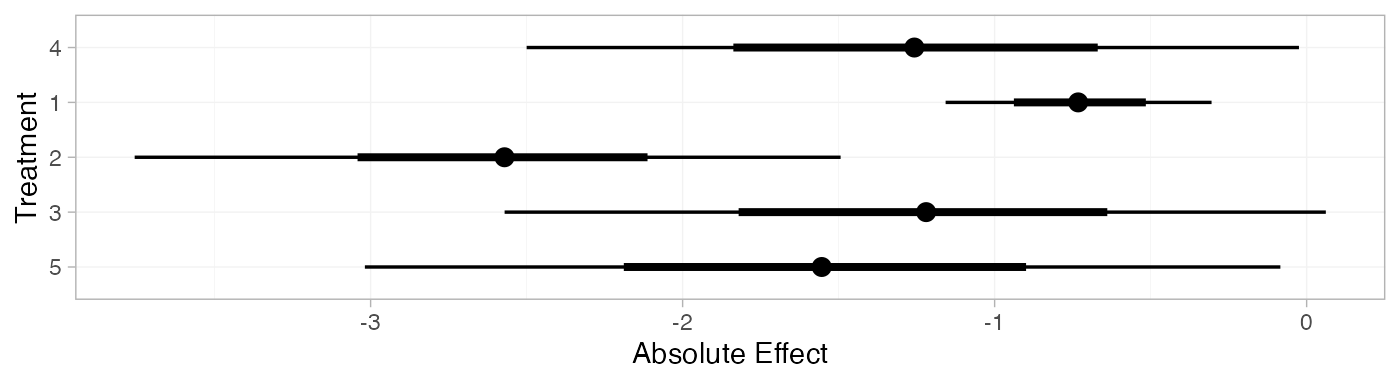

If the baseline argument is omitted, predictions of mean off-time reduction will be produced for every study in the network based on their estimated baseline response $\mu_j$:

arm_pred_FE_studies <- predict(arm_fit_FE, type = "response")
arm_pred_FE_studies
#> ---------------------------------------------------------------------- Study: 1 ---- 
#> 
#>             mean   sd  2.5%   25%   50%   75% 97.5% Bulk_ESS Tail_ESS Rhat
#> pred[1: 4] -1.66 0.46 -2.52 -1.98 -1.66 -1.35 -0.77     1884     2597    1
#> pred[1: 1] -1.12 0.43 -1.97 -1.40 -1.12 -0.83 -0.27     3777     3318    1
#> pred[1: 2] -2.92 0.52 -3.97 -3.28 -2.92 -2.58 -1.93     3554     3227    1
#> pred[1: 3] -1.61 0.39 -2.35 -1.88 -1.61 -1.35 -0.85     3393     3380    1
#> pred[1: 5] -1.96 0.50 -2.90 -2.32 -1.97 -1.62 -0.95     2052     2630    1
#> 
#> ---------------------------------------------------------------------- Study: 2 ---- 
#> 
#>             mean   sd  2.5%   25%   50%   75% 97.5% Bulk_ESS Tail_ESS Rhat
#> pred[2: 4] -1.18 0.51 -2.16 -1.52 -1.18 -0.85 -0.17     1478     2006    1
#> pred[2: 1] -0.64 0.27 -1.16 -0.82 -0.64 -0.45 -0.12     4690     3456    1
#> pred[2: 2] -2.45 0.24 -2.91 -2.61 -2.45 -2.28 -1.99     5023     3477    1
#> pred[2: 3] -1.14 0.53 -2.17 -1.50 -1.14 -0.78 -0.10     2234     2653    1
#> pred[2: 5] -1.48 0.55 -2.55 -1.86 -1.49 -1.12 -0.38     1704     2387    1
#> 
#> ---------------------------------------------------------------------- Study: 3 ---- 
#> 
#>             mean   sd  2.5%   25%   50%   75% 97.5% Bulk_ESS Tail_ESS Rhat
#> pred[3: 4] -1.12 0.41 -1.93 -1.40 -1.12 -0.85 -0.31     1834     2637    1
#> pred[3: 1] -0.58 0.36 -1.26 -0.82 -0.58 -0.34  0.11     3935     3596    1
#> pred[3: 2] -2.39 0.37 -3.12 -2.64 -2.38 -2.14 -1.66     3721     3110    1
#> pred[3: 3] -1.08 0.48 -2.04 -1.40 -1.08 -0.75 -0.12     2759     2766    1
#> pred[3: 5] -1.43 0.47 -2.34 -1.74 -1.43 -1.11 -0.53     2144     2574    1
#> 
#> ---------------------------------------------------------------------- Study: 4 ---- 
#> 
#>             mean   sd  2.5%   25%   50%   75% 97.5% Bulk_ESS Tail_ESS Rhat
#> pred[4: 4] -0.39 0.30 -0.98 -0.60 -0.40 -0.19  0.21     2218     2451    1
#> pred[4: 1]  0.15 0.50 -0.85 -0.19  0.16  0.49  1.11     2290     2536    1
#> pred[4: 2] -1.66 0.56 -2.79 -2.03 -1.64 -1.28 -0.57     2160     2387    1
#> pred[4: 3] -0.35 0.25 -0.83 -0.52 -0.35 -0.18  0.14     5423     3545    1
#> pred[4: 5] -0.70 0.37 -1.42 -0.94 -0.70 -0.45  0.05     2540     2624    1
#> 
#> ---------------------------------------------------------------------- Study: 5 ---- 
#> 
#>             mean   sd  2.5%   25%   50%   75% 97.5% Bulk_ESS Tail_ESS Rhat
#> pred[5: 4] -0.56 0.34 -1.24 -0.79 -0.56 -0.33  0.10     2436     2809    1
#> pred[5: 1] -0.02 0.52 -1.03 -0.38 -0.01  0.33  0.99     2383     2706    1
#> pred[5: 2] -1.83 0.58 -2.94 -2.21 -1.84 -1.44 -0.71     2259     2744    1
#> pred[5: 3] -0.52 0.29 -1.08 -0.72 -0.53 -0.32  0.08     5745     3401    1
#> pred[5: 5] -0.87 0.41 -1.68 -1.14 -0.85 -0.58 -0.08     2827     2930    1
#> 
#> ---------------------------------------------------------------------- Study: 6 ---- 
#> 
#>             mean   sd  2.5%   25%   50%   75% 97.5% Bulk_ESS Tail_ESS Rhat
#> pred[6: 4] -2.20 0.18 -2.56 -2.32 -2.19 -2.08 -1.84     3387     2923    1
#> pred[6: 1] -1.65 0.50 -2.64 -1.99 -1.65 -1.32 -0.65     1650     2421    1
#> pred[6: 2] -3.46 0.55 -4.55 -3.83 -3.46 -3.09 -2.38     1680     2233    1
#> pred[6: 3] -2.15 0.38 -2.90 -2.40 -2.15 -1.89 -1.42     2186     2773    1
#> pred[6: 5] -2.50 0.17 -2.83 -2.61 -2.50 -2.38 -2.16     4987     3117    1
#> 
#> ---------------------------------------------------------------------- Study: 7 ---- 
#> 
#>             mean   sd  2.5%   25%   50%   75% 97.5% Bulk_ESS Tail_ESS Rhat
#> pred[7: 4] -1.80 0.18 -2.16 -1.92 -1.80 -1.68 -1.45     3551     2946    1
#> pred[7: 1] -1.26 0.50 -2.24 -1.59 -1.25 -0.91 -0.29     1679     2355    1
#> pred[7: 2] -3.06 0.55 -4.15 -3.43 -3.06 -2.70 -1.99     1742     2606    1
#> pred[7: 3] -1.75 0.38 -2.50 -2.01 -1.75 -1.50 -1.01     2214     2539    1
#> pred[7: 5] -2.10 0.21 -2.50 -2.24 -2.10 -1.96 -1.70     4914     3210    1
plot(arm_pred_FE_studies)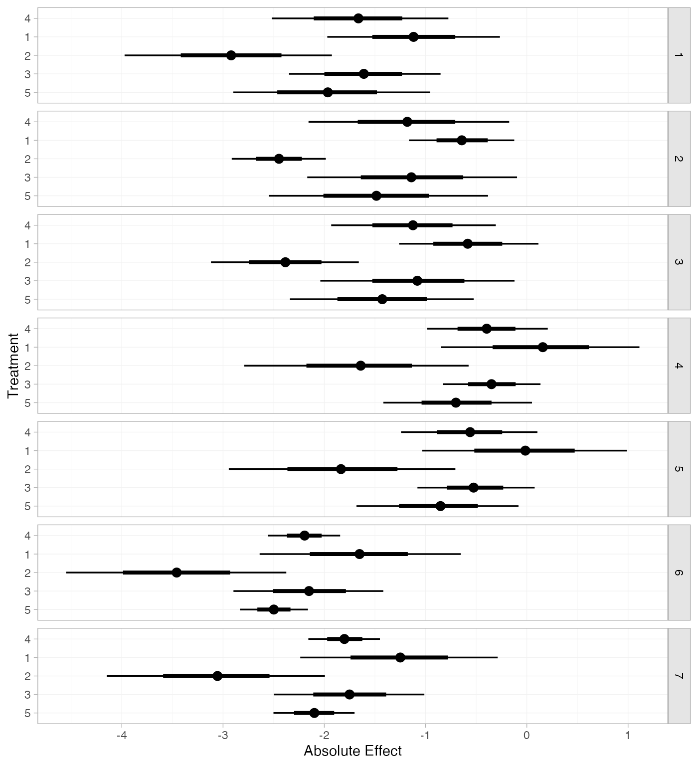

We can also produce treatment rankings, rank probabilities, and cumulative rank probabilities.

(arm_ranks <- posterior_ranks(arm_fit_FE))
#>         mean   sd 2.5% 25% 50% 75% 97.5% Bulk_ESS Tail_ESS Rhat
#> rank[4] 3.49 0.70    2   3   3   4     5     1990       NA    1
#> rank[1] 4.66 0.75    2   5   5   5     5     2335       NA    1
#> rank[2] 1.06 0.30    1   1   1   1     2     2583     2595    1
#> rank[3] 3.51 0.93    2   3   4   4     5     2854       NA    1
#> rank[5] 2.28 0.69    1   2   2   2     4     2545     2543    1
plot(arm_ranks)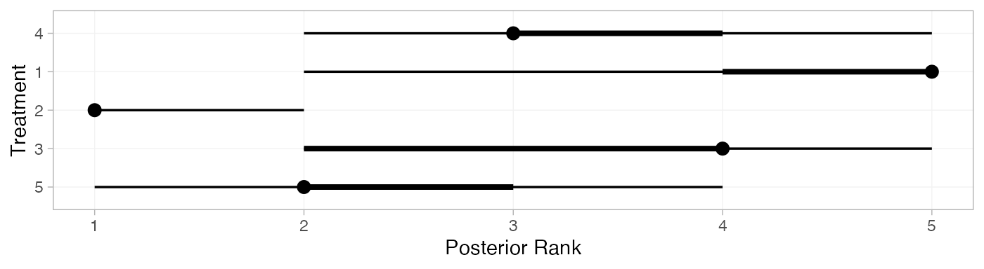

(arm_rankprobs <- posterior_rank_probs(arm_fit_FE))
#>      p_rank[1] p_rank[2] p_rank[3] p_rank[4] p_rank[5]
#> d[4]      0.00      0.04      0.49      0.39      0.07
#> d[1]      0.00      0.04      0.06      0.11      0.79
#> d[2]      0.95      0.04      0.01      0.00      0.00
#> d[3]      0.00      0.17      0.26      0.45      0.12
#> d[5]      0.04      0.71      0.18      0.05      0.01
plot(arm_rankprobs)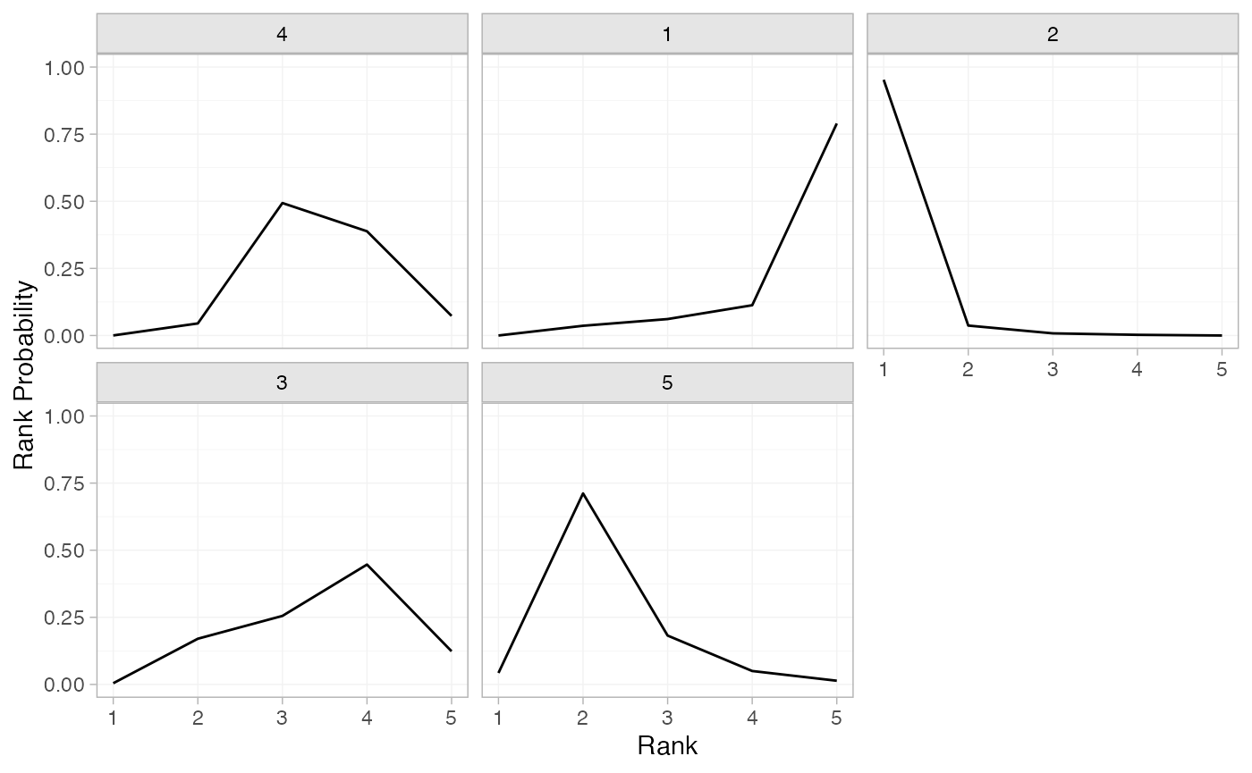

(arm_cumrankprobs <- posterior_rank_probs(arm_fit_FE, cumulative = TRUE))
#>      p_rank[1] p_rank[2] p_rank[3] p_rank[4] p_rank[5]
#> d[4]      0.00      0.05      0.54      0.93         1
#> d[1]      0.00      0.04      0.10      0.21         1
#> d[2]      0.95      0.99      1.00      1.00         1
#> d[3]      0.00      0.17      0.43      0.88         1
#> d[5]      0.04      0.75      0.94      0.99         1
plot(arm_cumrankprobs)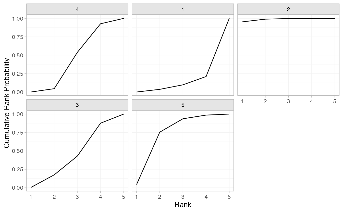

Analysis of contrast-based data

We now perform an analysis using the contrast-based data (mean differences and standard errors).

Setting up the network

With contrast-level data giving the mean difference in off-time reduction (diff) and standard error (se_diff), we use the function set_agd_contrast() to set up the network.

contr_net <- set_agd_contrast(parkinsons, 
                              study = studyn,
                              trt = trtn,
                              y = diff, 
                              se = se_diff,
                              sample_size = n)
contr_net
#> A network with 7 AgD studies (contrast-based).
#> 
#> -------------------------------------------------- AgD studies (contrast-based) ---- 
#>  Study Treatment arms
#>  1     2: 1 | 3      
#>  2     2: 1 | 2      
#>  3     3: 4 | 1 | 2  
#>  4     2: 4 | 3      
#>  5     2: 4 | 3      
#>  6     2: 4 | 5      
#>  7     2: 4 | 5      
#> 
#>  Outcome type: continuous
#> ------------------------------------------------------------------------------------
#> Total number of treatments: 5
#> Total number of studies: 7
#> Reference treatment is: 4
#> Network is connected

The sample_size argument is optional, but enables the nodes to be weighted by sample size in the network plot.

Plot the network structure.

plot(contr_net, weight_edges = TRUE, weight_nodes = TRUE)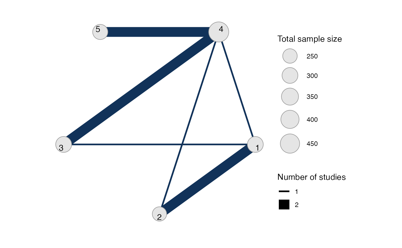

Meta-analysis models

We fit both fixed effect (FE) and random effects (RE) models.

Fixed effect meta-analysis

First, we fit a fixed effect model using the nma() function with trt_effects = "fixed". We use $\mathrm{N}(0, 100^2)$ prior distributions for the treatment effects $d_k$. We can examine the range of parameter values implied by these prior distributions with the summary() method:

summary(normal(scale = 100))
#> A Normal prior distribution: location = 0, scale = 100.
#> 50% of the prior density lies between -67.45 and 67.45.
#> 95% of the prior density lies between -196 and 196.

The model is fitted using the nma() function.

contr_fit_FE <- nma(contr_net, 
                    trt_effects = "fixed",
                    prior_trt = normal(scale = 100))
#> Note: Setting "4" as the network reference treatment.

Basic parameter summaries are given by the print() method:

contr_fit_FE
#> A fixed effects NMA with a normal likelihood (identity link).
#> Inference for Stan model: normal.
#> 4 chains, each with iter=2000; warmup=1000; thin=1; 
#> post-warmup draws per chain=1000, total post-warmup draws=4000.
#> 
#>       mean se_mean   sd  2.5%   25%   50%   75% 97.5% n_eff Rhat
#> d[1]  0.54    0.01 0.46 -0.37  0.23  0.53  0.84  1.43  2175    1
#> d[2] -1.27    0.01 0.50 -2.26 -1.62 -1.27 -0.93 -0.29  2263    1
#> d[3]  0.05    0.01 0.33 -0.58 -0.18  0.05  0.27  0.71  3058    1
#> d[5] -0.30    0.00 0.21 -0.71 -0.44 -0.30 -0.16  0.08  3831    1
#> lp__ -3.12    0.03 1.36 -6.55 -3.77 -2.82 -2.12 -1.39  1841    1
#> 
#> Samples were drawn using NUTS(diag_e) at Tue Sep 24 09:07:54 2024.
#> For each parameter, n_eff is a crude measure of effective sample size,
#> and Rhat is the potential scale reduction factor on split chains (at 
#> convergence, Rhat=1).

The prior and posterior distributions can be compared visually using the plot_prior_posterior() function:

plot_prior_posterior(contr_fit_FE)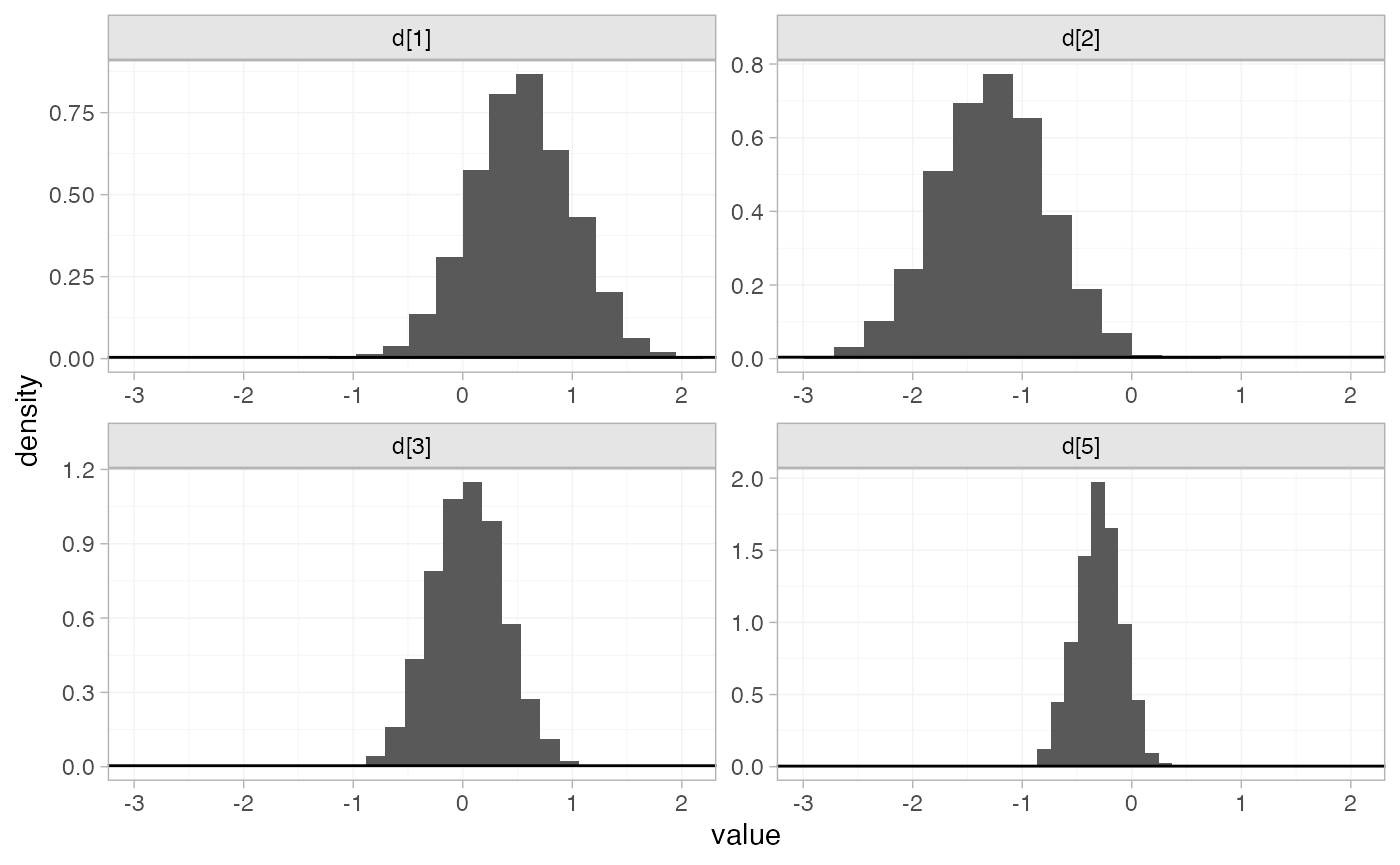

Random effects meta-analysis

We now fit a random effects model using the nma() function with trt_effects = "random". Again, we use $\mathrm{N}(0, 100^2)$ prior distributions for the treatment effects $d_k$, and we additionally use a $\textrm{half-N}(5^2)$ prior for the heterogeneity standard deviation $\tau$. We can examine the range of parameter values implied by these prior distributions with the summary() method:

summary(normal(scale = 100))
#> A Normal prior distribution: location = 0, scale = 100.
#> 50% of the prior density lies between -67.45 and 67.45.
#> 95% of the prior density lies between -196 and 196.
summary(half_normal(scale = 5))
#> A half-Normal prior distribution: location = 0, scale = 5.
#> 50% of the prior density lies between 0 and 3.37.
#> 95% of the prior density lies between 0 and 9.8.

Fitting the RE model

contr_fit_RE <- nma(contr_net, 
                    seed = 1150676438,
                    trt_effects = "random",
                    prior_trt = normal(scale = 100),
                    prior_het = half_normal(scale = 5),
                    adapt_delta = 0.99)
#> Note: Setting "4" as the network reference treatment.

We do see a small number of divergent transition errors, which cannot simply be removed by increasing the value of the adapt_delta argument (by default set to 0.95 for RE models). To diagnose, we use the pairs() method to investigate where in the posterior distribution these divergences are happening (indicated by red crosses):

pairs(contr_fit_RE, pars = c("d[3]", "delta[4: 4 vs. 3]", "tau"))

The divergent transitions occur in the upper tail of the heterogeneity standard deviation. In this case, with only a small number of studies, there is not very much information to estimate the heterogeneity standard deviation and the prior distribution may be too heavy-tailed. We could consider a more informative prior distribution for the heterogeneity variance to aid estimation.

Basic parameter summaries are given by the print() method:

contr_fit_RE
#> A random effects NMA with a normal likelihood (identity link).
#> Inference for Stan model: normal.
#> 4 chains, each with iter=2000; warmup=1000; thin=1; 
#> post-warmup draws per chain=1000, total post-warmup draws=4000.
#> 
#>       mean se_mean   sd   2.5%    25%   50%   75% 97.5% n_eff Rhat
#> d[1]  0.51    0.01 0.60  -0.65   0.13  0.52  0.90  1.65  2435 1.00
#> d[2] -1.33    0.01 0.69  -2.70  -1.74 -1.31 -0.89 -0.01  2356 1.00
#> d[3]  0.03    0.01 0.47  -0.83  -0.24  0.03  0.30  0.95  1953 1.00
#> d[5] -0.31    0.01 0.41  -1.19  -0.52 -0.30 -0.10  0.48  2077 1.00
#> lp__ -8.27    0.09 2.92 -14.84 -10.03 -7.97 -6.20 -3.43  1172 1.00
#> tau   0.38    0.01 0.38   0.01   0.12  0.28  0.52  1.42   945 1.01
#> 
#> Samples were drawn using NUTS(diag_e) at Tue Sep 24 09:07:57 2024.
#> For each parameter, n_eff is a crude measure of effective sample size,
#> and Rhat is the potential scale reduction factor on split chains (at 
#> convergence, Rhat=1).

By default, summaries of the study-specific relative effects $\delta_{jk}$ are hidden, but could be examined by changing the pars argument:

# Not run
print(contr_fit_RE, pars = c("d", "delta"))

The prior and posterior distributions can be compared visually using the plot_prior_posterior() function:

plot_prior_posterior(contr_fit_RE)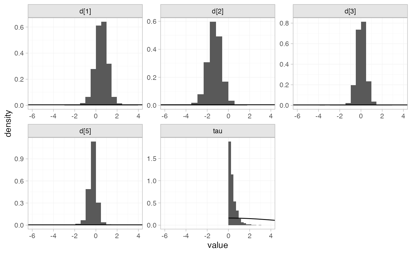

Model comparison

Model fit can be checked using the dic() function:

(contr_dic_FE <- dic(contr_fit_FE))
#> Residual deviance: 6.2 (on 8 data points)
#>                pD: 3.9
#>               DIC: 10.2

(contr_dic_RE <- dic(contr_fit_RE))
#> Residual deviance: 6.5 (on 8 data points)
#>                pD: 5.3
#>               DIC: 11.8

Both models fit the data well, having posterior mean residual deviance close to the number of data points. The DIC is similar between models, so we choose the FE model based on parsimony.

We can also examine the residual deviance contributions with the corresponding plot() method.

plot(contr_dic_FE)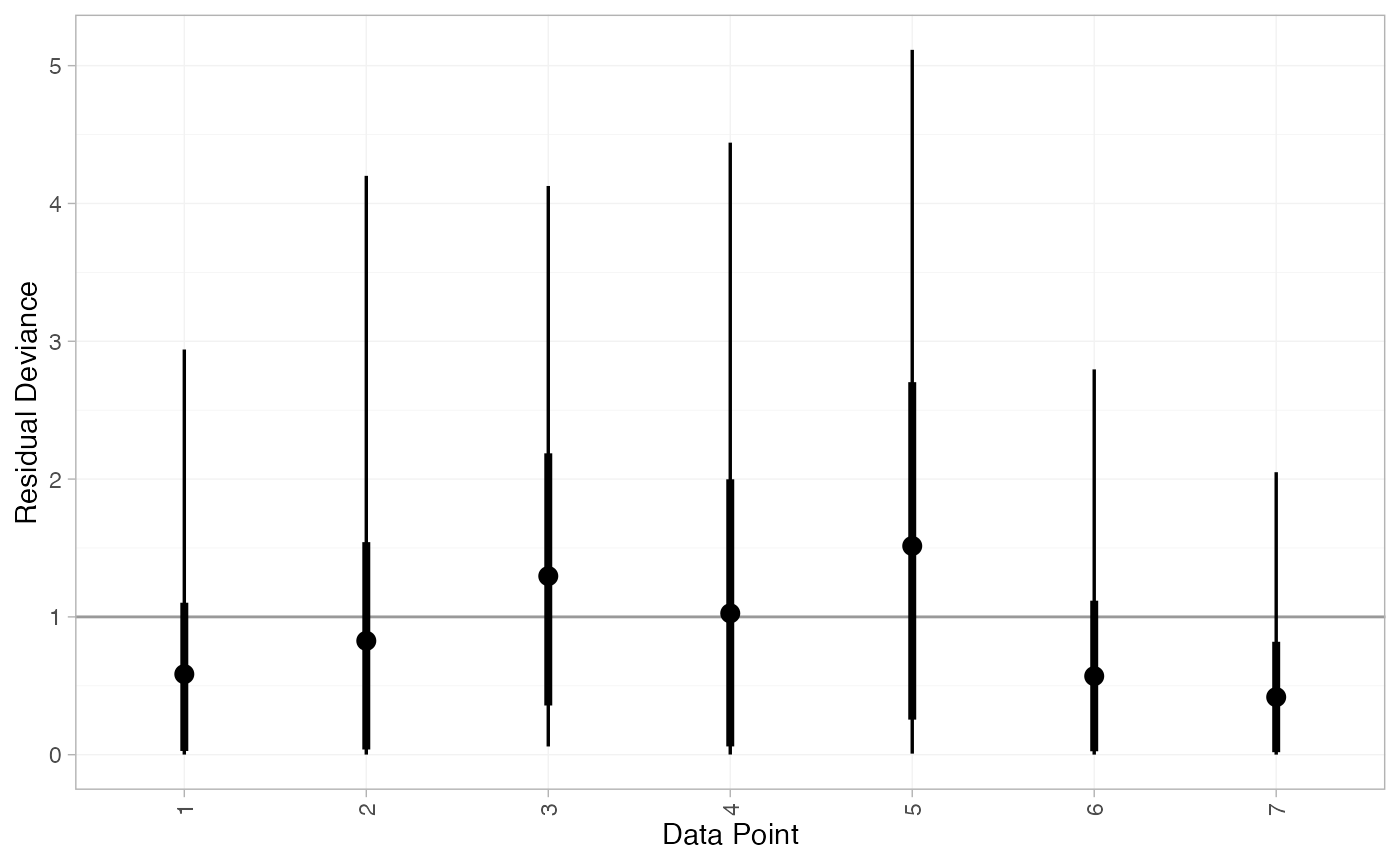

plot(contr_dic_RE)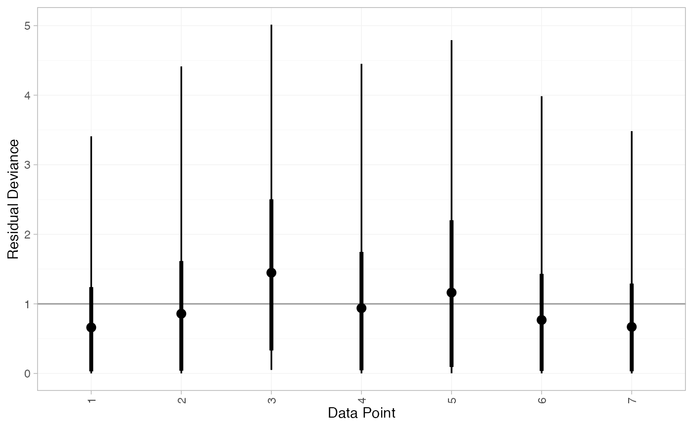

Further results

For comparison with Dias et al. (2011), we can produce relative effects against placebo using the relative_effects() function with trt_ref = 1:

(contr_releff_FE <- relative_effects(contr_fit_FE, trt_ref = 1))
#>       mean   sd  2.5%   25%   50%   75% 97.5% Bulk_ESS Tail_ESS Rhat
#> d[4] -0.54 0.46 -1.43 -0.84 -0.53 -0.23  0.37     2193     2485    1
#> d[2] -1.81 0.33 -2.46 -2.03 -1.81 -1.58 -1.17     5584     3277    1
#> d[3] -0.49 0.48 -1.43 -0.81 -0.48 -0.15  0.46     3041     2924    1
#> d[5] -0.83 0.50 -1.83 -1.18 -0.83 -0.50  0.15     2444     2494    1
plot(contr_releff_FE, ref_line = 0)

(contr_releff_RE <- relative_effects(contr_fit_RE, trt_ref = 1))
#>       mean   sd  2.5%   25%   50%   75% 97.5% Bulk_ESS Tail_ESS Rhat
#> d[4] -0.51 0.60 -1.65 -0.90 -0.52 -0.13  0.65     2505     2312    1
#> d[2] -1.84 0.51 -2.85 -2.12 -1.83 -1.55 -0.87     3437     2322    1
#> d[3] -0.48 0.63 -1.71 -0.86 -0.49 -0.11  0.75     3210     2479    1
#> d[5] -0.82 0.74 -2.29 -1.25 -0.82 -0.38  0.59     2325     1876    1
plot(contr_releff_RE, ref_line = 0)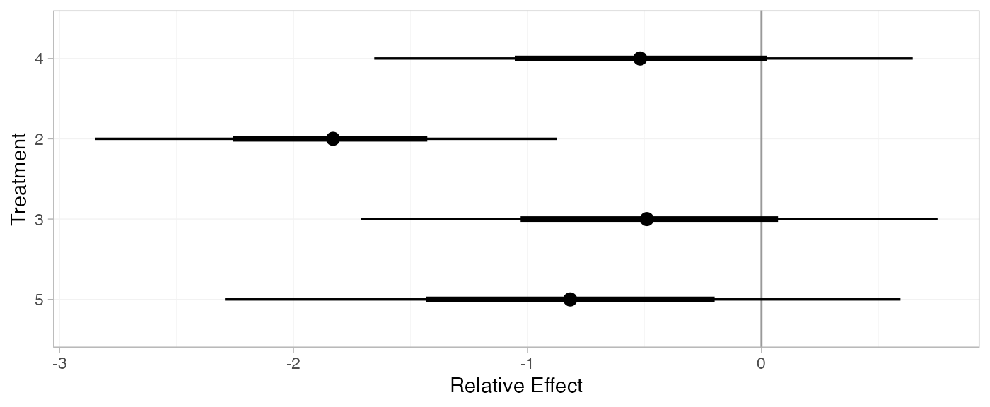

Following Dias et al. (2011), we produce absolute predictions of the mean off-time reduction on each treatment assuming a Normal distribution for the outcomes on treatment 1 (placebo) with mean $-0.73$ and precision $21$. We use the predict() method, where the baseline argument takes a distr() distribution object with which we specify the corresponding Normal distribution, and we specify baseline_trt = 1 to indicate that the baseline distribution corresponds to treatment 1. (Strictly speaking, type = "response" is unnecessary here, since the identity link function was used.)

contr_pred_FE <- predict(contr_fit_FE, 
                       baseline = distr(qnorm, mean = -0.73, sd = 21^-0.5),
                       type = "response",
                       baseline_trt = 1)
contr_pred_FE
#>          mean   sd  2.5%   25%   50%   75% 97.5% Bulk_ESS Tail_ESS Rhat
#> pred[4] -1.26 0.51 -2.27 -1.61 -1.27 -0.91 -0.25     2343     3040    1
#> pred[1] -0.73 0.22 -1.16 -0.88 -0.73 -0.58 -0.30     3988     3629    1
#> pred[2] -2.54 0.39 -3.33 -2.80 -2.54 -2.28 -1.77     4860     3667    1
#> pred[3] -1.22 0.53 -2.24 -1.58 -1.22 -0.87 -0.18     3029     3222    1
#> pred[5] -1.56 0.55 -2.65 -1.94 -1.56 -1.19 -0.51     2499     2945    1
plot(contr_pred_FE)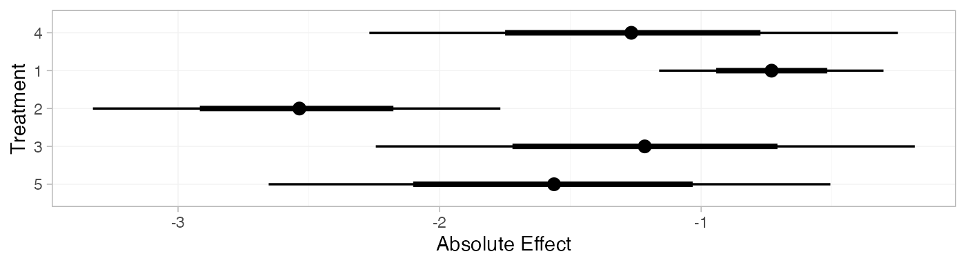

contr_pred_RE <- predict(contr_fit_RE, 
                       baseline = distr(qnorm, mean = -0.73, sd = 21^-0.5),
                       type = "response",
                       baseline_trt = 1)
contr_pred_RE
#>          mean   sd  2.5%   25%   50%   75% 97.5% Bulk_ESS Tail_ESS Rhat
#> pred[4] -1.25 0.63 -2.47 -1.65 -1.25 -0.84 -0.01     2628     2267    1
#> pred[1] -0.73 0.22 -1.16 -0.88 -0.73 -0.59 -0.31     3715     3592    1
#> pred[2] -2.58 0.55 -3.67 -2.91 -2.58 -2.24 -1.50     3516     2575    1
#> pred[3] -1.22 0.67 -2.51 -1.63 -1.22 -0.80  0.09     3217     2295    1
#> pred[5] -1.56 0.77 -3.09 -2.02 -1.55 -1.09 -0.04     2445     2093    1
plot(contr_pred_RE)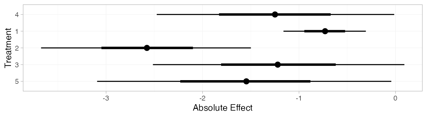

If the baseline argument is omitted an error will be raised, as there are no study baselines estimated in this network.

# Not run
predict(contr_fit_FE, type = "response")

We can also produce treatment rankings, rank probabilities, and cumulative rank probabilities.

(contr_ranks <- posterior_ranks(contr_fit_FE))
#>         mean   sd 2.5% 25% 50% 75% 97.5% Bulk_ESS Tail_ESS Rhat
#> rank[4] 3.49 0.70    2   3   3   4     5     2741       NA    1
#> rank[1] 4.68 0.73    2   5   5   5     5     2532       NA    1
#> rank[2] 1.04 0.23    1   1   1   1     2     2825     2834    1
#> rank[3] 3.51 0.92    2   3   4   4     5     3397       NA    1
#> rank[5] 2.28 0.65    1   2   2   2     4     2845     2127    1
plot(contr_ranks)

(contr_rankprobs <- posterior_rank_probs(contr_fit_FE))
#>      p_rank[1] p_rank[2] p_rank[3] p_rank[4] p_rank[5]
#> d[4]      0.00      0.04      0.50      0.39      0.07
#> d[1]      0.00      0.03      0.06      0.11      0.80
#> d[2]      0.96      0.03      0.00      0.00      0.00
#> d[3]      0.00      0.17      0.25      0.45      0.12
#> d[5]      0.03      0.72      0.19      0.05      0.01
plot(contr_rankprobs)

(contr_cumrankprobs <- posterior_rank_probs(contr_fit_FE, cumulative = TRUE))
#>      p_rank[1] p_rank[2] p_rank[3] p_rank[4] p_rank[5]
#> d[4]      0.00      0.04      0.54      0.93         1
#> d[1]      0.00      0.03      0.09      0.20         1
#> d[2]      0.96      0.99      1.00      1.00         1
#> d[3]      0.00      0.18      0.43      0.88         1
#> d[5]      0.03      0.75      0.94      0.99         1
plot(contr_cumrankprobs)

Analysis of mixed arm-based and contrast-based data

We now perform an analysis where some studies contribute arm-based data, and other contribute contrast-based data. Replicating Dias et al. (2011), we consider arm-based data from studies 1-3, and contrast-based data from studies 4-7.

studies <- parkinsons$studyn
(parkinsons_arm <- parkinsons[studies %in% 1:3, ])
#>   studyn trtn     y    se   n  diff se_diff
#> 1      1    1 -1.22 0.504  54    NA   0.504
#> 2      1    3 -1.53 0.439  95 -0.31   0.668
#> 3      2    1 -0.70 0.282 172    NA   0.282
#> 4      2    2 -2.40 0.258 173 -1.70   0.382
#> 5      3    1 -0.30 0.505  76    NA   0.505
#> 6      3    2 -2.60 0.510  71 -2.30   0.718
#> 7      3    4 -1.20 0.478  81 -0.90   0.695
(parkinsons_contr <- parkinsons[studies %in% 4:7, ])
#>    studyn trtn     y    se   n  diff se_diff
#> 8       4    3 -0.24 0.265 128    NA   0.265
#> 9       4    4 -0.59 0.354  72 -0.35   0.442
#> 10      5    3 -0.73 0.335  80    NA   0.335
#> 11      5    4 -0.18 0.442  46  0.55   0.555
#> 12      6    4 -2.20 0.197 137    NA   0.197
#> 13      6    5 -2.50 0.190 131 -0.30   0.274
#> 14      7    4 -1.80 0.200 154    NA   0.200
#> 15      7    5 -2.10 0.250 143 -0.30   0.320

Setting up the network

We use the functions set_agd_arm() and set_agd_contrast() to set up the respective data sources within the network, and then combine together with combine_network().

mix_arm_net <- set_agd_arm(parkinsons_arm, 
                           study = studyn,
                           trt = trtn,
                           y = y, 
                           se = se,
                           sample_size = n)

mix_contr_net <- set_agd_contrast(parkinsons_contr, 
                                  study = studyn,
                                  trt = trtn,
                                  y = diff, 
                                  se = se_diff,
                                  sample_size = n)

mix_net <- combine_network(mix_arm_net, mix_contr_net)
mix_net
#> A network with 3 AgD studies (arm-based), and 4 AgD studies (contrast-based).
#> 
#> ------------------------------------------------------- AgD studies (arm-based) ---- 
#>  Study Treatment arms
#>  1     2: 1 | 3      
#>  2     2: 1 | 2      
#>  3     3: 4 | 1 | 2  
#> 
#>  Outcome type: continuous
#> -------------------------------------------------- AgD studies (contrast-based) ---- 
#>  Study Treatment arms
#>  4     2: 4 | 3      
#>  5     2: 4 | 3      
#>  6     2: 4 | 5      
#>  7     2: 4 | 5      
#> 
#>  Outcome type: continuous
#> ------------------------------------------------------------------------------------
#> Total number of treatments: 5
#> Total number of studies: 7
#> Reference treatment is: 4
#> Network is connected

The sample_size argument is optional, but enables the nodes to be weighted by sample size in the network plot.

Plot the network structure.

plot(mix_net, weight_edges = TRUE, weight_nodes = TRUE)

Meta-analysis models

We fit both fixed effect (FE) and random effects (RE) models.

Fixed effect meta-analysis

First, we fit a fixed effect model using the nma() function with trt_effects = "fixed". We use $\mathrm{N}(0, 100^2)$ prior distributions for the treatment effects $d_k$ and study-specific intercepts $\mu_j$. We can examine the range of parameter values implied by these prior distributions with the summary() method:

summary(normal(scale = 100))
#> A Normal prior distribution: location = 0, scale = 100.
#> 50% of the prior density lies between -67.45 and 67.45.
#> 95% of the prior density lies between -196 and 196.

The model is fitted using the nma() function.

mix_fit_FE <- nma(mix_net, 
                  trt_effects = "fixed",
                  prior_intercept = normal(scale = 100),
                  prior_trt = normal(scale = 100))
#> Note: Setting "4" as the network reference treatment.

Basic parameter summaries are given by the print() method:

mix_fit_FE
#> A fixed effects NMA with a normal likelihood (identity link).
#> Inference for Stan model: normal.
#> 4 chains, each with iter=2000; warmup=1000; thin=1; 
#> post-warmup draws per chain=1000, total post-warmup draws=4000.
#> 
#>       mean se_mean   sd  2.5%   25%   50%   75% 97.5% n_eff Rhat
#> d[1]  0.51    0.01 0.48 -0.43  0.18  0.50  0.83  1.46  1586    1
#> d[2] -1.31    0.01 0.53 -2.35 -1.66 -1.31 -0.94 -0.31  1626    1
#> d[3]  0.04    0.01 0.32 -0.62 -0.18  0.04  0.26  0.64  2553    1
#> d[5] -0.30    0.00 0.21 -0.72 -0.44 -0.29 -0.16  0.11  3050    1
#> lp__ -4.66    0.05 1.87 -9.12 -5.73 -4.34 -3.23 -2.01  1640    1
#> 
#> Samples were drawn using NUTS(diag_e) at Tue Sep 24 09:08:02 2024.
#> For each parameter, n_eff is a crude measure of effective sample size,
#> and Rhat is the potential scale reduction factor on split chains (at 
#> convergence, Rhat=1).

By default, summaries of the study-specific intercepts $\mu_j$ are hidden, but could be examined by changing the pars argument:

# Not run
print(mix_fit_FE, pars = c("d", "mu"))

The prior and posterior distributions can be compared visually using the plot_prior_posterior() function:

plot_prior_posterior(mix_fit_FE)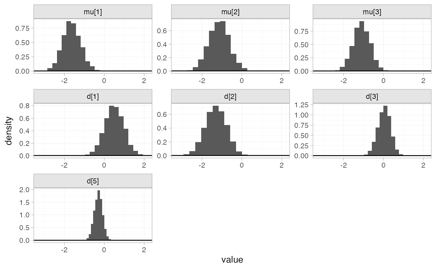

Random effects meta-analysis

We now fit a random effects model using the nma() function with trt_effects = "random". Again, we use $\mathrm{N}(0, 100^2)$ prior distributions for the treatment effects $d_k$ and study-specific intercepts $\mu_j$, and we additionally use a $\textrm{half-N}(5^2)$ prior for the heterogeneity standard deviation $\tau$. We can examine the range of parameter values implied by these prior distributions with the summary() method:

summary(normal(scale = 100))
#> A Normal prior distribution: location = 0, scale = 100.
#> 50% of the prior density lies between -67.45 and 67.45.
#> 95% of the prior density lies between -196 and 196.
summary(half_normal(scale = 5))
#> A half-Normal prior distribution: location = 0, scale = 5.
#> 50% of the prior density lies between 0 and 3.37.
#> 95% of the prior density lies between 0 and 9.8.

Fitting the RE model

mix_fit_RE <- nma(mix_net, 
                  seed = 437219664,
                  trt_effects = "random",
                  prior_intercept = normal(scale = 100),
                  prior_trt = normal(scale = 100),
                  prior_het = half_normal(scale = 5),
                  adapt_delta = 0.99)
#> Note: Setting "4" as the network reference treatment.

We do see a small number of divergent transition errors, which cannot simply be removed by increasing the value of the adapt_delta argument (by default set to 0.95 for RE models). To diagnose, we use the pairs() method to investigate where in the posterior distribution these divergences are happening (indicated by red crosses):

pairs(mix_fit_RE, pars = c("d[3]", "delta[4: 4 vs. 3]", "tau"))

The divergent transitions occur in the upper tail of the heterogeneity standard deviation. In this case, with only a small number of studies, there is not very much information to estimate the heterogeneity standard deviation and the prior distribution may be too heavy-tailed. We could consider a more informative prior distribution for the heterogeneity variance to aid estimation.

Basic parameter summaries are given by the print() method:

mix_fit_RE
#> A random effects NMA with a normal likelihood (identity link).
#> Inference for Stan model: normal.
#> 4 chains, each with iter=2000; warmup=1000; thin=1; 
#> post-warmup draws per chain=1000, total post-warmup draws=4000.
#> 
#>        mean se_mean   sd   2.5%    25%    50%   75% 97.5% n_eff Rhat
#> d[1]   0.55    0.01 0.59  -0.61   0.15   0.54  0.91  1.73  1945    1
#> d[2]  -1.30    0.01 0.67  -2.61  -1.73  -1.29 -0.88  0.01  2026    1
#> d[3]   0.03    0.01 0.45  -0.86  -0.24   0.02  0.30  0.92  2923    1
#> d[5]  -0.31    0.01 0.40  -1.13  -0.51  -0.30 -0.09  0.47  2330    1
#> lp__ -10.88    0.09 3.26 -18.03 -12.90 -10.60 -8.59 -5.26  1465    1
#> tau    0.37    0.01 0.36   0.01   0.12   0.27  0.49  1.28  1080    1
#> 
#> Samples were drawn using NUTS(diag_e) at Tue Sep 24 09:08:06 2024.
#> For each parameter, n_eff is a crude measure of effective sample size,
#> and Rhat is the potential scale reduction factor on split chains (at 
#> convergence, Rhat=1).

By default, summaries of the study-specific intercepts $\mu_j$ and study-specific relative effects $\delta_{jk}$ are hidden, but could be examined by changing the pars argument:

# Not run
print(mix_fit_RE, pars = c("d", "mu", "delta"))

The prior and posterior distributions can be compared visually using the plot_prior_posterior() function:

plot_prior_posterior(mix_fit_RE)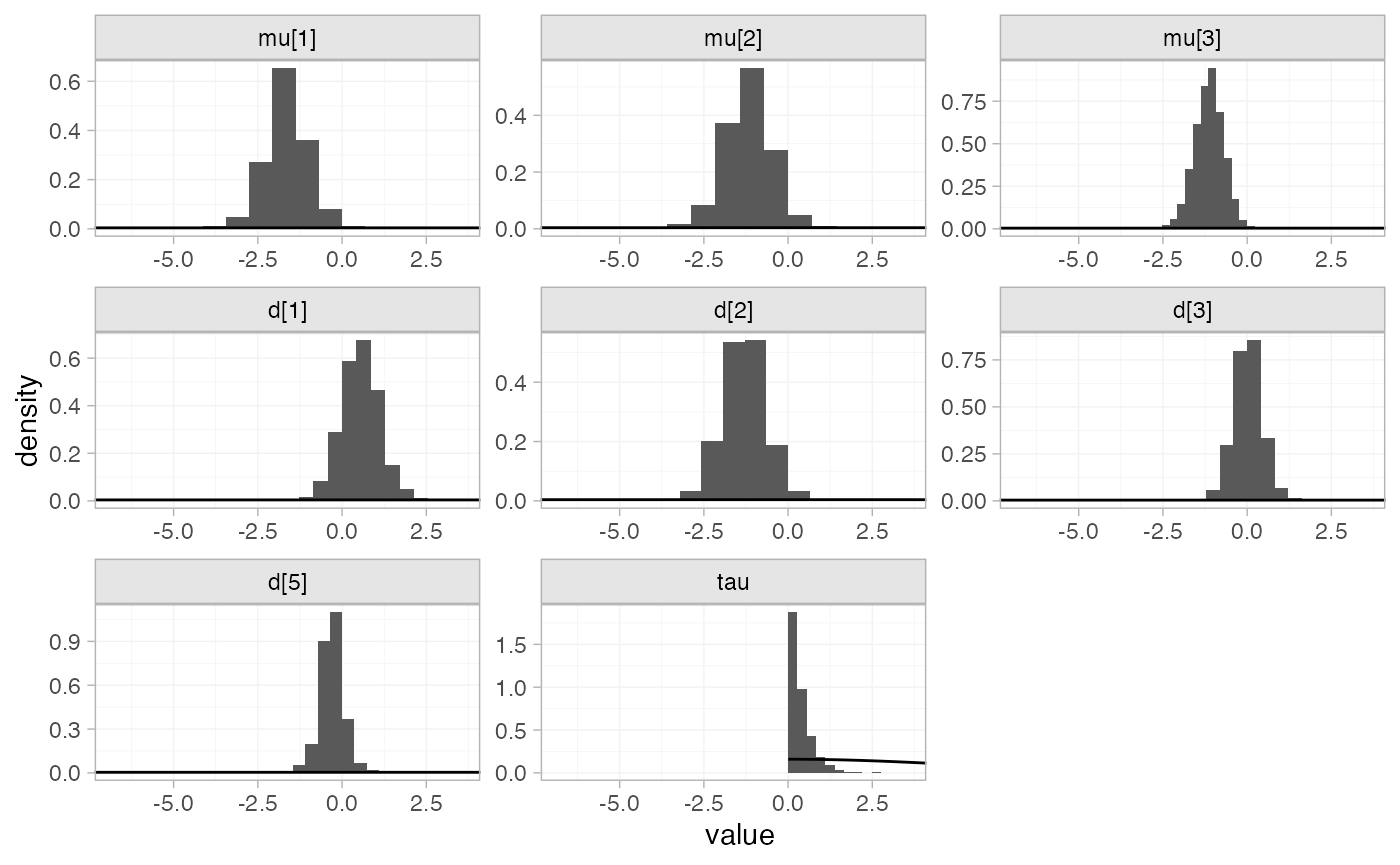

Model comparison

Model fit can be checked using the dic() function:

(mix_dic_FE <- dic(mix_fit_FE))
#> Residual deviance: 9.3 (on 11 data points)
#>                pD: 7
#>               DIC: 16.3

(mix_dic_RE <- dic(mix_fit_RE))
#> Residual deviance: 9.6 (on 11 data points)
#>                pD: 8.4
#>               DIC: 18

Both models fit the data well, having posterior mean residual deviance close to the number of data points. The DIC is similar between models, so we choose the FE model based on parsimony.

We can also examine the residual deviance contributions with the corresponding plot() method.

plot(mix_dic_FE)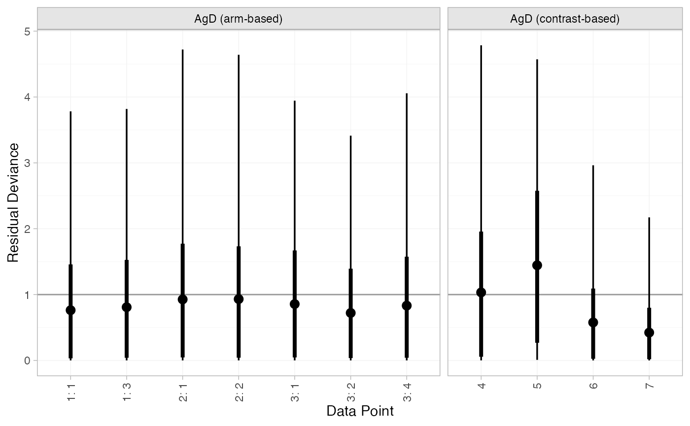

plot(mix_dic_RE)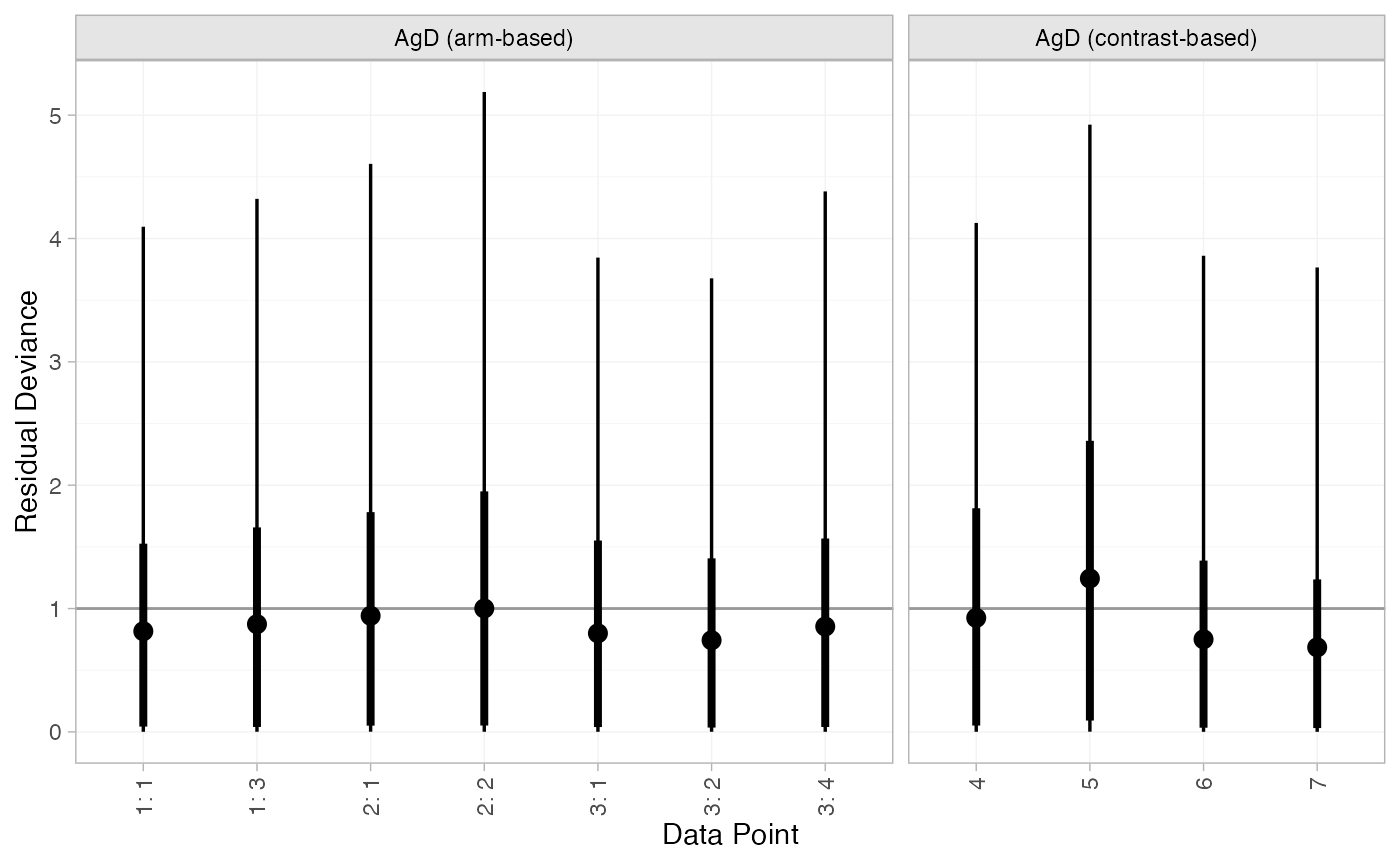

Further results

For comparison with Dias et al. (2011), we can produce relative effects against placebo using the relative_effects() function with trt_ref = 1:

(mix_releff_FE <- relative_effects(mix_fit_FE, trt_ref = 1))
#>       mean   sd  2.5%   25%   50%   75% 97.5% Bulk_ESS Tail_ESS Rhat
#> d[4] -0.51 0.48 -1.46 -0.83 -0.50 -0.18  0.43     1606     2262    1
#> d[2] -1.81 0.33 -2.47 -2.04 -1.81 -1.58 -1.16     5739     2842    1
#> d[3] -0.47 0.49 -1.43 -0.80 -0.47 -0.14  0.50     2409     3011    1
#> d[5] -0.80 0.53 -1.85 -1.16 -0.79 -0.45  0.27     1713     2275    1
plot(mix_releff_FE, ref_line = 0)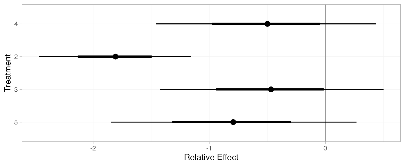

(mix_releff_RE <- relative_effects(mix_fit_RE, trt_ref = 1))
#>       mean   sd  2.5%   25%   50%   75% 97.5% Bulk_ESS Tail_ESS Rhat
#> d[4] -0.55 0.59 -1.73 -0.91 -0.54 -0.15  0.61     1952     2171    1
#> d[2] -1.85 0.49 -2.89 -2.13 -1.85 -1.55 -0.96     4054     2813    1
#> d[3] -0.52 0.62 -1.74 -0.89 -0.51 -0.13  0.64     2989     2480    1
#> d[5] -0.85 0.71 -2.23 -1.28 -0.84 -0.40  0.51     2067     1959    1
plot(mix_releff_RE, ref_line = 0)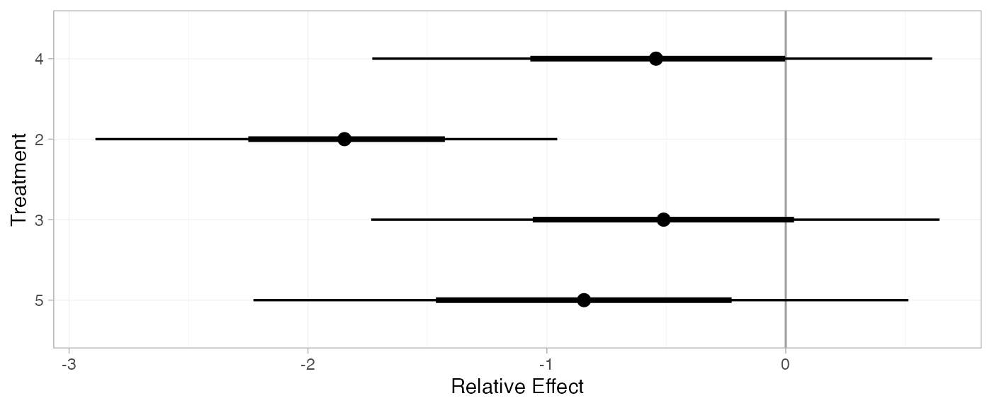

Following Dias et al. (2011), we produce absolute predictions of the mean off-time reduction on each treatment assuming a Normal distribution for the outcomes on treatment 1 (placebo) with mean $-0.73$ and precision $21$. We use the predict() method, where the baseline argument takes a distr() distribution object with which we specify the corresponding Normal distribution, and we specify baseline_trt = 1 to indicate that the baseline distribution corresponds to treatment 1. (Strictly speaking, type = "response" is unnecessary here, since the identity link function was used.)

mix_pred_FE <- predict(mix_fit_FE, 
                       baseline = distr(qnorm, mean = -0.73, sd = 21^-0.5),
                       type = "response",
                       baseline_trt = 1)
mix_pred_FE
#>          mean   sd  2.5%   25%   50%   75% 97.5% Bulk_ESS Tail_ESS Rhat
#> pred[4] -1.23 0.53 -2.27 -1.59 -1.22 -0.88 -0.17     1777     2613    1
#> pred[1] -0.72 0.22 -1.14 -0.87 -0.72 -0.58 -0.29     3556     3638    1
#> pred[2] -2.53 0.39 -3.31 -2.80 -2.53 -2.26 -1.78     5108     3551    1
#> pred[3] -1.19 0.54 -2.24 -1.55 -1.21 -0.82 -0.10     2525     3106    1
#> pred[5] -1.52 0.57 -2.66 -1.91 -1.52 -1.14 -0.37     1842     2382    1
plot(mix_pred_FE)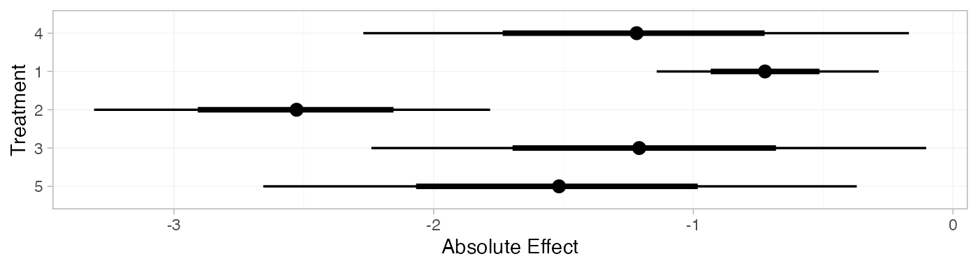

mix_pred_RE <- predict(mix_fit_RE, 
                       baseline = distr(qnorm, mean = -0.73, sd = 21^-0.5),
                       type = "response",
                       baseline_trt = 1)
mix_pred_RE
#>          mean   sd  2.5%   25%   50%   75% 97.5% Bulk_ESS Tail_ESS Rhat
#> pred[4] -1.27 0.63 -2.52 -1.68 -1.27 -0.87 -0.06     2088     2415    1
#> pred[1] -0.73 0.22 -1.17 -0.88 -0.73 -0.58 -0.31     4051     3817    1
#> pred[2] -2.58 0.54 -3.68 -2.90 -2.57 -2.24 -1.57     4000     2896    1
#> pred[3] -1.25 0.65 -2.52 -1.66 -1.24 -0.84  0.01     3099     2869    1
#> pred[5] -1.58 0.74 -2.99 -2.04 -1.58 -1.14 -0.13     2124     2509    1
plot(mix_pred_RE)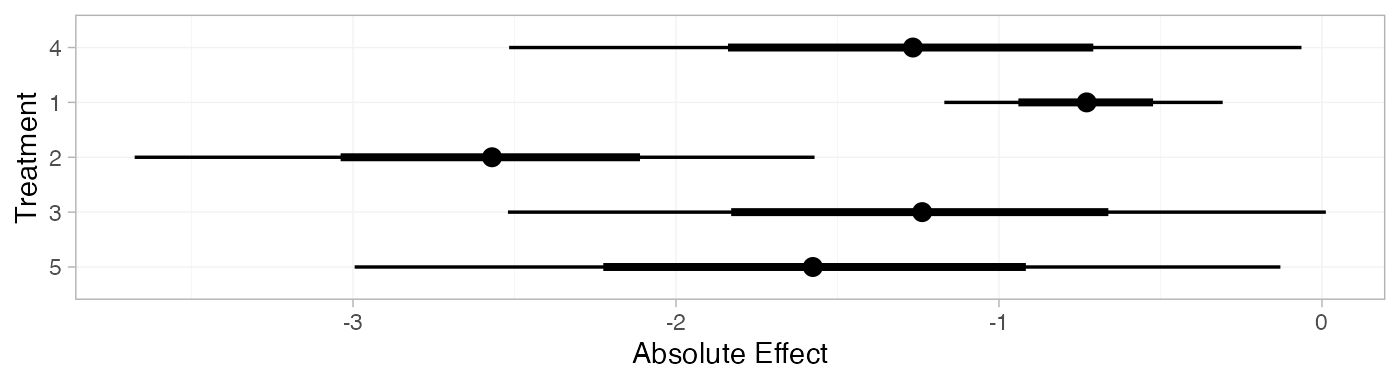

If the baseline argument is omitted, predictions of mean off-time reduction will be produced for every arm-based study in the network based on their estimated baseline response $\mu_j$:

mix_pred_FE_studies <- predict(mix_fit_FE, type = "response")
mix_pred_FE_studies
#> ---------------------------------------------------------------------- Study: 1 ---- 
#> 
#>             mean   sd  2.5%   25%   50%   75% 97.5% Bulk_ESS Tail_ESS Rhat
#> pred[1: 4] -1.64 0.45 -2.50 -1.94 -1.65 -1.34 -0.70     2068     2403    1
#> pred[1: 1] -1.13 0.43 -1.95 -1.42 -1.14 -0.84 -0.29     3407     2920    1
#> pred[1: 2] -2.94 0.52 -3.93 -3.29 -2.94 -2.59 -1.96     3148     3019    1
#> pred[1: 3] -1.60 0.39 -2.35 -1.86 -1.61 -1.34 -0.84     3552     3294    1
#> pred[1: 5] -1.93 0.50 -2.88 -2.28 -1.93 -1.60 -0.94     2099     2516    1
#> 
#> ---------------------------------------------------------------------- Study: 2 ---- 
#> 
#>             mean   sd  2.5%   25%   50%   75% 97.5% Bulk_ESS Tail_ESS Rhat
#> pred[2: 4] -1.14 0.52 -2.14 -1.50 -1.13 -0.79 -0.10     1589     2167    1
#> pred[2: 1] -0.64 0.26 -1.15 -0.81 -0.63 -0.46 -0.11     4656     3462    1
#> pred[2: 2] -2.45 0.24 -2.93 -2.61 -2.45 -2.28 -1.96     5173     3692    1
#> pred[2: 3] -1.11 0.53 -2.15 -1.46 -1.11 -0.74 -0.05     2303     2812    1
#> pred[2: 5] -1.44 0.56 -2.53 -1.83 -1.44 -1.05 -0.31     1690     2295    1
#> 
#> ---------------------------------------------------------------------- Study: 3 ---- 
#> 
#>             mean   sd  2.5%   25%   50%   75% 97.5% Bulk_ESS Tail_ESS Rhat
#> pred[3: 4] -1.10 0.42 -1.94 -1.38 -1.10 -0.81 -0.28     2007     2612    1
#> pred[3: 1] -0.59 0.36 -1.30 -0.84 -0.60 -0.35  0.11     4337     2979    1
#> pred[3: 2] -2.41 0.39 -3.17 -2.66 -2.41 -2.14 -1.66     3882     3167    1
#> pred[3: 3] -1.06 0.47 -1.99 -1.39 -1.04 -0.75 -0.14     3112     2988    1
#> pred[3: 5] -1.40 0.48 -2.34 -1.71 -1.40 -1.06 -0.47     2072     2409    1
plot(mix_pred_FE_studies)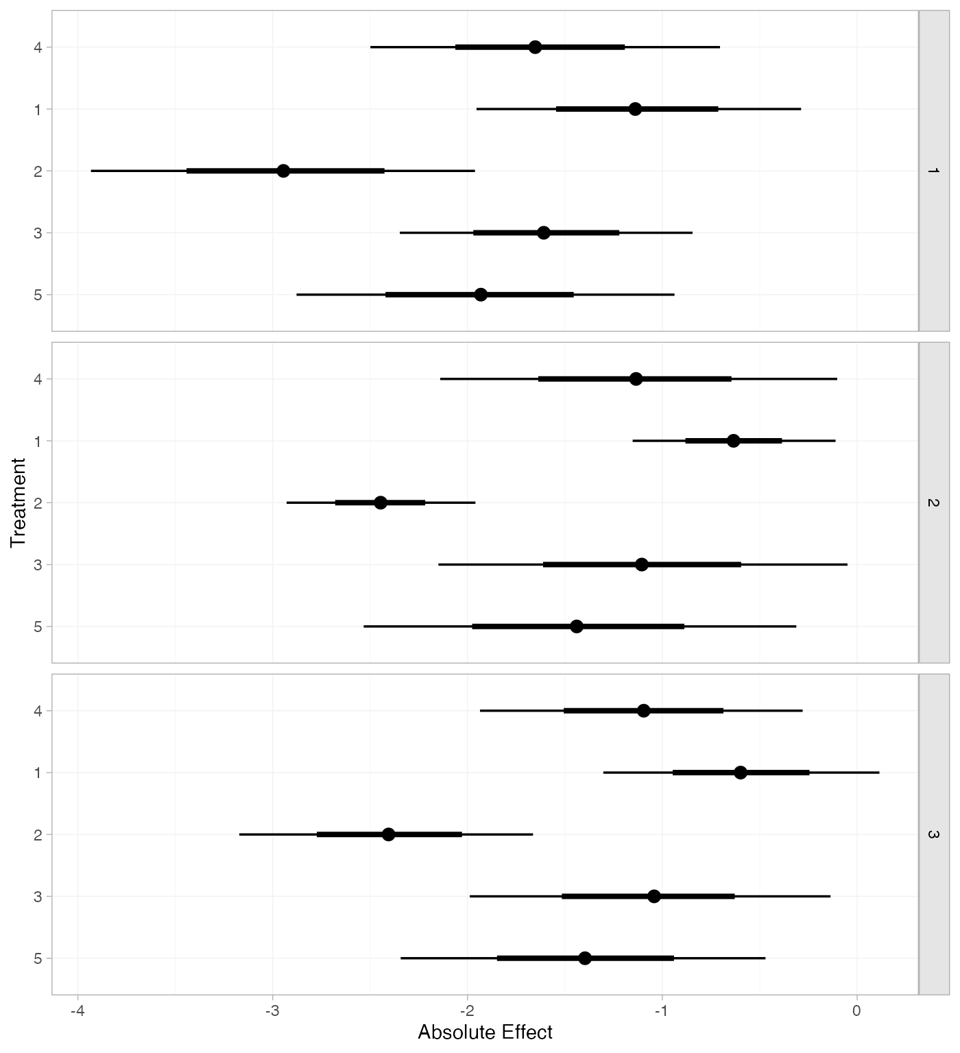

We can also produce treatment rankings, rank probabilities, and cumulative rank probabilities.

(mix_ranks <- posterior_ranks(mix_fit_FE))
#>         mean   sd 2.5% 25% 50% 75% 97.5% Bulk_ESS Tail_ESS Rhat
#> rank[4] 3.51 0.71    2   3   3   4     5     2379       NA    1
#> rank[1] 4.63 0.79    2   5   5   5     5     2077       NA    1
#> rank[2] 1.05 0.26    1   1   1   1     2     2572     2682    1
#> rank[3] 3.52 0.92    2   3   4   4     5     3397       NA    1
#> rank[5] 2.29 0.68    1   2   2   3     4     2517     2745    1
plot(mix_ranks)

(mix_rankprobs <- posterior_rank_probs(mix_fit_FE))
#>      p_rank[1] p_rank[2] p_rank[3] p_rank[4] p_rank[5]
#> d[4]      0.00      0.04      0.49      0.39      0.08
#> d[1]      0.00      0.04      0.07      0.11      0.78
#> d[2]      0.96      0.03      0.01      0.00      0.00
#> d[3]      0.00      0.17      0.25      0.45      0.13
#> d[5]      0.04      0.71      0.19      0.05      0.01
plot(mix_rankprobs)

(mix_cumrankprobs <- posterior_rank_probs(mix_fit_FE, cumulative = TRUE))
#>      p_rank[1] p_rank[2] p_rank[3] p_rank[4] p_rank[5]
#> d[4]      0.00      0.04      0.53      0.92         1
#> d[1]      0.00      0.04      0.11      0.22         1
#> d[2]      0.96      0.99      1.00      1.00         1
#> d[3]      0.00      0.17      0.43      0.87         1
#> d[5]      0.04      0.75      0.94      0.99         1
plot(mix_cumrankprobs)

References

Dias, S., N. J. Welton, A. J. Sutton, and A. E. Ades. 2011. “NICE DSU Technical Support Document 2: A Generalised Linear Modelling Framework for Pair-Wise and Network Meta-Analysis of Randomised Controlled Trials.” National Institute for Health and Care Excellence. https://www.sheffield.ac.uk/nice-dsu.