Generate (population-average) relative treatment effects. If a ML-NMR or meta-regression model was fitted, these are specific to each study population.
Usage
relative_effects(
  x,
  newdata = NULL,
  study = NULL,
  all_contrasts = FALSE,
  trt_ref = NULL,
  probs = c(0.025, 0.25, 0.5, 0.75, 0.975),
  predictive_distribution = FALSE,
  summary = TRUE
)
Arguments
- x
A
stan_nmaobject created bynma()- newdata
Only used if a regression model is fitted. A data frame of study details, one row per study, giving the covariate values at which to produce relative effects. Column names must match variables in the regression model. If
NULL, relative effects are produced for all studies in the network.- study
Column of
newdatawhich specifies study names, otherwise studies will be labelled by row number.- all_contrasts
Logical, generate estimates for all contrasts (
TRUE), or just the "basic" contrasts against the network reference treatment (FALSE)? DefaultFALSE.- trt_ref
Reference treatment to construct relative effects against, if
all_contrasts = FALSE. By default, relative effects will be against the network reference treatment. Coerced to character string.- probs
Numeric vector of quantiles of interest to present in computed summary, default
c(0.025, 0.25, 0.5, 0.75, 0.975)- predictive_distribution
Logical, when a random effects model has been fitted, should the predictive distribution for relative effects in a new study be returned? Default
FALSE.- summary
Logical, calculate posterior summaries? Default
TRUE.
Value
A nma_summary object if summary = TRUE, otherwise a list
containing a 3D MCMC array of samples and (for regression models) a data
frame of study information.
See also
plot.nma_summary() for plotting the relative effects.
Examples
## Smoking cessation
# \donttest{
# Run smoking RE NMA example if not already available
if (!exists("smk_fit_RE")) example("example_smk_re", run.donttest = TRUE)
# }
# \donttest{
# Produce relative effects
smk_releff_RE <- relative_effects(smk_fit_RE)
smk_releff_RE
#> mean sd 2.5% 25% 50% 75% 97.5% Bulk_ESS
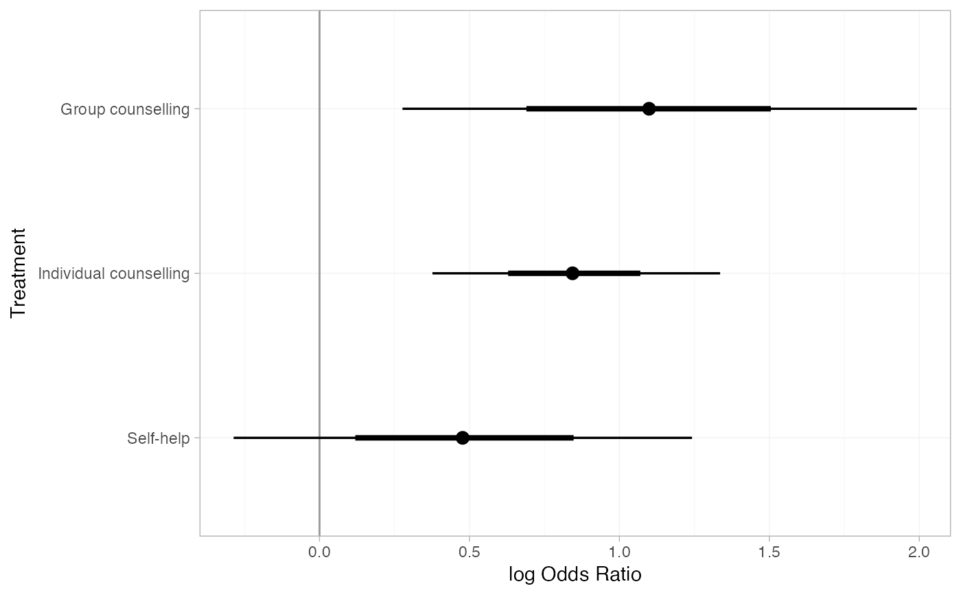
#> d[Group counselling] 1.08 0.42 0.24 0.81 1.08 1.34 1.93 1927
#> d[Individual counselling] 0.83 0.24 0.37 0.67 0.82 0.99 1.34 1173
#> d[Self-help] 0.50 0.40 -0.29 0.24 0.49 0.76 1.32 1990
#> Tail_ESS Rhat
#> d[Group counselling] 2122 1
#> d[Individual counselling] 1735 1
#> d[Self-help] 2528 1
plot(smk_releff_RE, ref_line = 0)
 # Relative effects for all pairwise comparisons
relative_effects(smk_fit_RE, all_contrasts = TRUE)
#> mean sd 2.5% 25% 50%
#> d[Group counselling vs. No intervention] 1.08 0.42 0.24 0.81 1.08
#> d[Individual counselling vs. No intervention] 0.83 0.24 0.37 0.67 0.82
#> d[Self-help vs. No intervention] 0.50 0.40 -0.29 0.24 0.49
#> d[Individual counselling vs. Group counselling] -0.25 0.40 -1.03 -0.51 -0.25
#> d[Self-help vs. Group counselling] -0.58 0.47 -1.48 -0.90 -0.58
#> d[Self-help vs. Individual counselling] -0.33 0.40 -1.11 -0.58 -0.34
#> 75% 97.5% Bulk_ESS Tail_ESS
#> d[Group counselling vs. No intervention] 1.34 1.93 1927 2122
#> d[Individual counselling vs. No intervention] 0.99 1.34 1173 1735
#> d[Self-help vs. No intervention] 0.76 1.32 1990 2528
#> d[Individual counselling vs. Group counselling] 0.02 0.54 2698 2503
#> d[Self-help vs. Group counselling] -0.28 0.38 3019 2749
#> d[Self-help vs. Individual counselling] -0.07 0.47 2311 2468
#> Rhat
#> d[Group counselling vs. No intervention] 1
#> d[Individual counselling vs. No intervention] 1
#> d[Self-help vs. No intervention] 1
#> d[Individual counselling vs. Group counselling] 1
#> d[Self-help vs. Group counselling] 1
#> d[Self-help vs. Individual counselling] 1
# Relative effects against a different reference treatment
relative_effects(smk_fit_RE, trt_ref = "Self-help")
#> mean sd 2.5% 25% 50% 75% 97.5% Bulk_ESS
#> d[No intervention] -0.50 0.40 -1.32 -0.76 -0.49 -0.24 0.29 1990
#> d[Group counselling] 0.58 0.47 -0.38 0.28 0.58 0.90 1.48 3019
#> d[Individual counselling] 0.33 0.40 -0.47 0.07 0.34 0.58 1.11 2311
#> Tail_ESS Rhat
#> d[No intervention] 2528 1
#> d[Group counselling] 2749 1
#> d[Individual counselling] 2468 1
# Transforming to odds ratios
# We work with the array of relative effects samples
LOR_array <- as.array(smk_releff_RE)
OR_array <- exp(LOR_array)
# mcmc_array objects can be summarised to produce a nma_summary object
smk_OR_RE <- summary(OR_array)
# This can then be printed or plotted
smk_OR_RE
#> mean sd 2.5% 25% 50% 75% 97.5% Bulk_ESS Tail_ESS
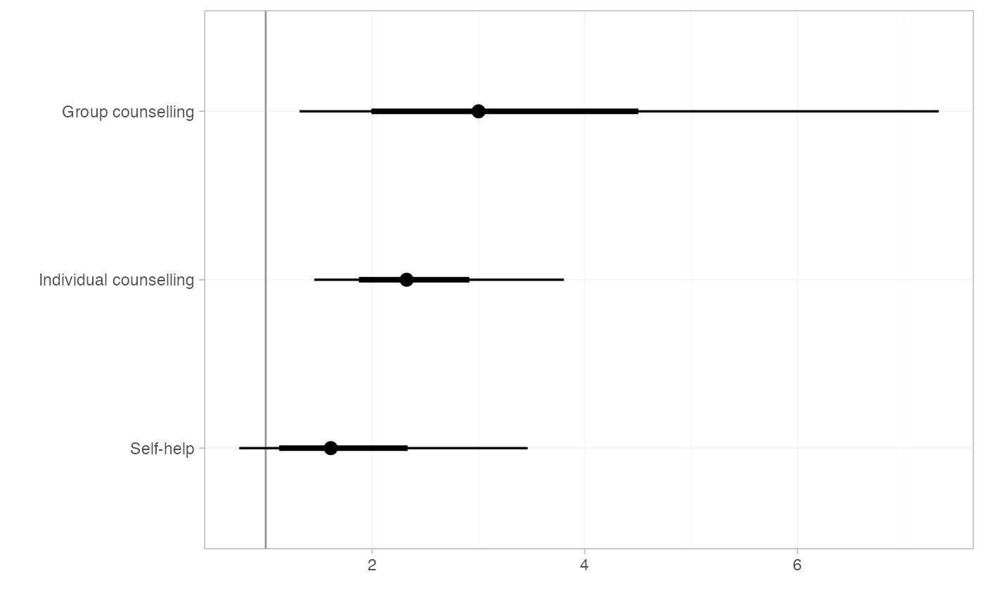
#> d[Group counselling] 3.22 1.51 1.27 2.24 2.94 3.82 6.89 1927 2122
#> d[Individual counselling] 2.37 0.61 1.44 1.96 2.28 2.68 3.80 1173 1735
#> d[Self-help] 1.79 0.77 0.75 1.27 1.63 2.14 3.73 1990 2528
#> Rhat
#> d[Group counselling] 1
#> d[Individual counselling] 1
#> d[Self-help] 1
plot(smk_OR_RE, ref_line = 1)
# Relative effects for all pairwise comparisons
relative_effects(smk_fit_RE, all_contrasts = TRUE)
#> mean sd 2.5% 25% 50%
#> d[Group counselling vs. No intervention] 1.08 0.42 0.24 0.81 1.08
#> d[Individual counselling vs. No intervention] 0.83 0.24 0.37 0.67 0.82
#> d[Self-help vs. No intervention] 0.50 0.40 -0.29 0.24 0.49
#> d[Individual counselling vs. Group counselling] -0.25 0.40 -1.03 -0.51 -0.25
#> d[Self-help vs. Group counselling] -0.58 0.47 -1.48 -0.90 -0.58
#> d[Self-help vs. Individual counselling] -0.33 0.40 -1.11 -0.58 -0.34
#> 75% 97.5% Bulk_ESS Tail_ESS
#> d[Group counselling vs. No intervention] 1.34 1.93 1927 2122
#> d[Individual counselling vs. No intervention] 0.99 1.34 1173 1735
#> d[Self-help vs. No intervention] 0.76 1.32 1990 2528
#> d[Individual counselling vs. Group counselling] 0.02 0.54 2698 2503
#> d[Self-help vs. Group counselling] -0.28 0.38 3019 2749
#> d[Self-help vs. Individual counselling] -0.07 0.47 2311 2468
#> Rhat
#> d[Group counselling vs. No intervention] 1
#> d[Individual counselling vs. No intervention] 1
#> d[Self-help vs. No intervention] 1
#> d[Individual counselling vs. Group counselling] 1
#> d[Self-help vs. Group counselling] 1
#> d[Self-help vs. Individual counselling] 1
# Relative effects against a different reference treatment
relative_effects(smk_fit_RE, trt_ref = "Self-help")
#> mean sd 2.5% 25% 50% 75% 97.5% Bulk_ESS
#> d[No intervention] -0.50 0.40 -1.32 -0.76 -0.49 -0.24 0.29 1990
#> d[Group counselling] 0.58 0.47 -0.38 0.28 0.58 0.90 1.48 3019
#> d[Individual counselling] 0.33 0.40 -0.47 0.07 0.34 0.58 1.11 2311
#> Tail_ESS Rhat
#> d[No intervention] 2528 1
#> d[Group counselling] 2749 1
#> d[Individual counselling] 2468 1
# Transforming to odds ratios
# We work with the array of relative effects samples
LOR_array <- as.array(smk_releff_RE)
OR_array <- exp(LOR_array)
# mcmc_array objects can be summarised to produce a nma_summary object
smk_OR_RE <- summary(OR_array)
# This can then be printed or plotted
smk_OR_RE
#> mean sd 2.5% 25% 50% 75% 97.5% Bulk_ESS Tail_ESS
#> d[Group counselling] 3.22 1.51 1.27 2.24 2.94 3.82 6.89 1927 2122
#> d[Individual counselling] 2.37 0.61 1.44 1.96 2.28 2.68 3.80 1173 1735
#> d[Self-help] 1.79 0.77 0.75 1.27 1.63 2.14 3.73 1990 2528
#> Rhat
#> d[Group counselling] 1
#> d[Individual counselling] 1
#> d[Self-help] 1
plot(smk_OR_RE, ref_line = 1)
 # }
## Plaque psoriasis ML-NMR
# \donttest{
# Run plaque psoriasis ML-NMR example if not already available
if (!exists("pso_fit")) example("example_pso_mlnmr", run.donttest = TRUE)
# }
# \donttest{
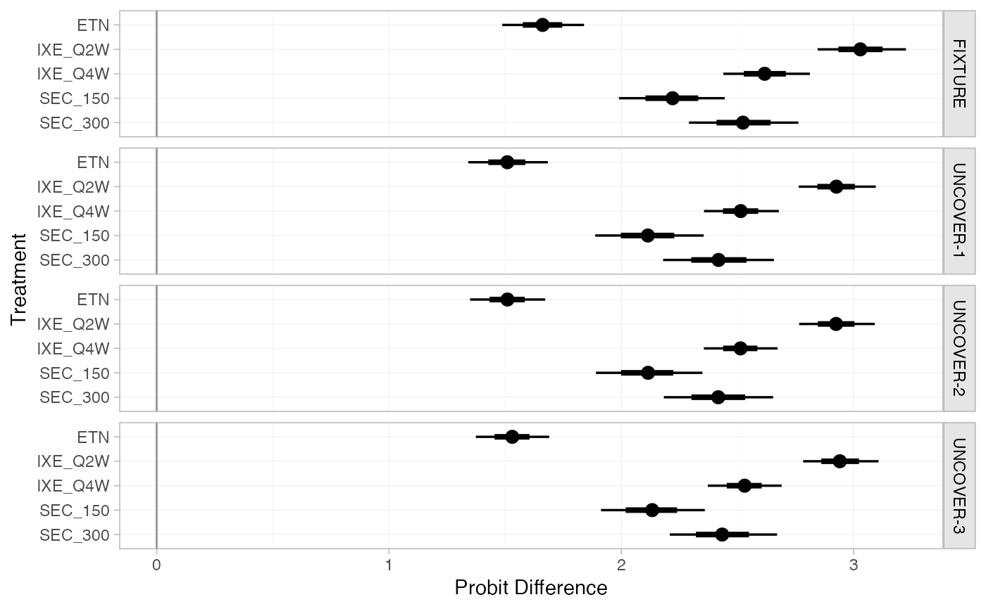
# Produce population-adjusted relative effects for all study populations in
# the network
pso_releff <- relative_effects(pso_fit)
pso_releff
#> ---------------------------------------------------------------- Study: FIXTURE ----
#>
#> Covariate values:
#> durnpso prevsys bsa weight psa
#> 1.6 0.62 0.34 8.34 0.14
#>
#> mean sd 2.5% 25% 50% 75% 97.5% Bulk_ESS Tail_ESS Rhat
#> d[FIXTURE: ETN] 1.66 0.09 1.49 1.60 1.66 1.72 1.83 4300 3436 1
#> d[FIXTURE: IXE_Q2W] 3.03 0.10 2.84 2.96 3.03 3.09 3.22 5509 3194 1
#> d[FIXTURE: IXE_Q4W] 2.62 0.09 2.44 2.55 2.61 2.67 2.80 5332 3525 1
#> d[FIXTURE: SEC_150] 2.22 0.12 1.98 2.14 2.22 2.30 2.45 4727 3599 1
#> d[FIXTURE: SEC_300] 2.53 0.12 2.29 2.44 2.53 2.61 2.76 5529 3542 1
#>
#> -------------------------------------------------------------- Study: UNCOVER-1 ----
#>
#> Covariate values:
#> durnpso prevsys bsa weight psa
#> 2 0.73 0.28 9.24 0.28
#>
#> mean sd 2.5% 25% 50% 75% 97.5% Bulk_ESS Tail_ESS
#> d[UNCOVER-1: ETN] 1.51 0.08 1.34 1.45 1.51 1.56 1.68 4586 3355
#> d[UNCOVER-1: IXE_Q2W] 2.92 0.09 2.75 2.86 2.92 2.98 3.10 5606 2840
#> d[UNCOVER-1: IXE_Q4W] 2.51 0.08 2.35 2.46 2.51 2.56 2.67 5852 3336
#> d[UNCOVER-1: SEC_150] 2.12 0.12 1.87 2.03 2.11 2.20 2.35 5375 3440
#> d[UNCOVER-1: SEC_300] 2.42 0.13 2.18 2.33 2.42 2.50 2.66 6240 3186
#> Rhat
#> d[UNCOVER-1: ETN] 1
#> d[UNCOVER-1: IXE_Q2W] 1
#> d[UNCOVER-1: IXE_Q4W] 1
#> d[UNCOVER-1: SEC_150] 1
#> d[UNCOVER-1: SEC_300] 1
#>
#> -------------------------------------------------------------- Study: UNCOVER-2 ----
#>
#> Covariate values:
#> durnpso prevsys bsa weight psa
#> 1.87 0.64 0.27 9.17 0.24
#>
#> mean sd 2.5% 25% 50% 75% 97.5% Bulk_ESS Tail_ESS
#> d[UNCOVER-2: ETN] 1.51 0.08 1.35 1.45 1.51 1.56 1.67 4632 3275
#> d[UNCOVER-2: IXE_Q2W] 2.92 0.09 2.75 2.86 2.92 2.98 3.09 5774 2898
#> d[UNCOVER-2: IXE_Q4W] 2.51 0.08 2.36 2.46 2.51 2.56 2.67 6223 3155
#> d[UNCOVER-2: SEC_150] 2.12 0.12 1.88 2.04 2.12 2.20 2.34 5363 3600
#> d[UNCOVER-2: SEC_300] 2.42 0.12 2.18 2.34 2.42 2.50 2.66 6336 3284
#> Rhat
#> d[UNCOVER-2: ETN] 1
#> d[UNCOVER-2: IXE_Q2W] 1
#> d[UNCOVER-2: IXE_Q4W] 1
#> d[UNCOVER-2: SEC_150] 1
#> d[UNCOVER-2: SEC_300] 1
#>
#> -------------------------------------------------------------- Study: UNCOVER-3 ----
#>
#> Covariate values:
#> durnpso prevsys bsa weight psa
#> 1.78 0.59 0.28 9.01 0.2
#>
#> mean sd 2.5% 25% 50% 75% 97.5% Bulk_ESS Tail_ESS
#> d[UNCOVER-3: ETN] 1.53 0.08 1.38 1.48 1.53 1.58 1.69 4655 3543
#> d[UNCOVER-3: IXE_Q2W] 2.94 0.09 2.77 2.88 2.94 3.00 3.11 5892 2903
#> d[UNCOVER-3: IXE_Q4W] 2.53 0.08 2.37 2.47 2.53 2.58 2.69 6007 3478
#> d[UNCOVER-3: SEC_150] 2.13 0.12 1.90 2.06 2.13 2.21 2.36 5263 3277
#> d[UNCOVER-3: SEC_300] 2.44 0.12 2.20 2.36 2.44 2.52 2.67 6272 3380
#> Rhat
#> d[UNCOVER-3: ETN] 1
#> d[UNCOVER-3: IXE_Q2W] 1
#> d[UNCOVER-3: IXE_Q4W] 1
#> d[UNCOVER-3: SEC_150] 1
#> d[UNCOVER-3: SEC_300] 1
#>
plot(pso_releff, ref_line = 0)
# }
## Plaque psoriasis ML-NMR
# \donttest{
# Run plaque psoriasis ML-NMR example if not already available
if (!exists("pso_fit")) example("example_pso_mlnmr", run.donttest = TRUE)
# }
# \donttest{
# Produce population-adjusted relative effects for all study populations in
# the network
pso_releff <- relative_effects(pso_fit)
pso_releff
#> ---------------------------------------------------------------- Study: FIXTURE ----
#>
#> Covariate values:
#> durnpso prevsys bsa weight psa
#> 1.6 0.62 0.34 8.34 0.14
#>
#> mean sd 2.5% 25% 50% 75% 97.5% Bulk_ESS Tail_ESS Rhat
#> d[FIXTURE: ETN] 1.66 0.09 1.49 1.60 1.66 1.72 1.83 4300 3436 1
#> d[FIXTURE: IXE_Q2W] 3.03 0.10 2.84 2.96 3.03 3.09 3.22 5509 3194 1
#> d[FIXTURE: IXE_Q4W] 2.62 0.09 2.44 2.55 2.61 2.67 2.80 5332 3525 1
#> d[FIXTURE: SEC_150] 2.22 0.12 1.98 2.14 2.22 2.30 2.45 4727 3599 1
#> d[FIXTURE: SEC_300] 2.53 0.12 2.29 2.44 2.53 2.61 2.76 5529 3542 1
#>
#> -------------------------------------------------------------- Study: UNCOVER-1 ----
#>
#> Covariate values:
#> durnpso prevsys bsa weight psa
#> 2 0.73 0.28 9.24 0.28
#>
#> mean sd 2.5% 25% 50% 75% 97.5% Bulk_ESS Tail_ESS
#> d[UNCOVER-1: ETN] 1.51 0.08 1.34 1.45 1.51 1.56 1.68 4586 3355
#> d[UNCOVER-1: IXE_Q2W] 2.92 0.09 2.75 2.86 2.92 2.98 3.10 5606 2840
#> d[UNCOVER-1: IXE_Q4W] 2.51 0.08 2.35 2.46 2.51 2.56 2.67 5852 3336
#> d[UNCOVER-1: SEC_150] 2.12 0.12 1.87 2.03 2.11 2.20 2.35 5375 3440
#> d[UNCOVER-1: SEC_300] 2.42 0.13 2.18 2.33 2.42 2.50 2.66 6240 3186
#> Rhat
#> d[UNCOVER-1: ETN] 1
#> d[UNCOVER-1: IXE_Q2W] 1
#> d[UNCOVER-1: IXE_Q4W] 1
#> d[UNCOVER-1: SEC_150] 1
#> d[UNCOVER-1: SEC_300] 1
#>
#> -------------------------------------------------------------- Study: UNCOVER-2 ----
#>
#> Covariate values:
#> durnpso prevsys bsa weight psa
#> 1.87 0.64 0.27 9.17 0.24
#>
#> mean sd 2.5% 25% 50% 75% 97.5% Bulk_ESS Tail_ESS
#> d[UNCOVER-2: ETN] 1.51 0.08 1.35 1.45 1.51 1.56 1.67 4632 3275
#> d[UNCOVER-2: IXE_Q2W] 2.92 0.09 2.75 2.86 2.92 2.98 3.09 5774 2898
#> d[UNCOVER-2: IXE_Q4W] 2.51 0.08 2.36 2.46 2.51 2.56 2.67 6223 3155
#> d[UNCOVER-2: SEC_150] 2.12 0.12 1.88 2.04 2.12 2.20 2.34 5363 3600
#> d[UNCOVER-2: SEC_300] 2.42 0.12 2.18 2.34 2.42 2.50 2.66 6336 3284
#> Rhat
#> d[UNCOVER-2: ETN] 1
#> d[UNCOVER-2: IXE_Q2W] 1
#> d[UNCOVER-2: IXE_Q4W] 1
#> d[UNCOVER-2: SEC_150] 1
#> d[UNCOVER-2: SEC_300] 1
#>
#> -------------------------------------------------------------- Study: UNCOVER-3 ----
#>
#> Covariate values:
#> durnpso prevsys bsa weight psa
#> 1.78 0.59 0.28 9.01 0.2
#>
#> mean sd 2.5% 25% 50% 75% 97.5% Bulk_ESS Tail_ESS
#> d[UNCOVER-3: ETN] 1.53 0.08 1.38 1.48 1.53 1.58 1.69 4655 3543
#> d[UNCOVER-3: IXE_Q2W] 2.94 0.09 2.77 2.88 2.94 3.00 3.11 5892 2903
#> d[UNCOVER-3: IXE_Q4W] 2.53 0.08 2.37 2.47 2.53 2.58 2.69 6007 3478
#> d[UNCOVER-3: SEC_150] 2.13 0.12 1.90 2.06 2.13 2.21 2.36 5263 3277
#> d[UNCOVER-3: SEC_300] 2.44 0.12 2.20 2.36 2.44 2.52 2.67 6272 3380
#> Rhat
#> d[UNCOVER-3: ETN] 1
#> d[UNCOVER-3: IXE_Q2W] 1
#> d[UNCOVER-3: IXE_Q4W] 1
#> d[UNCOVER-3: SEC_150] 1
#> d[UNCOVER-3: SEC_300] 1
#>
plot(pso_releff, ref_line = 0)
 # Produce population-adjusted relative effects for a different target
# population
new_agd_means <- data.frame(
bsa = 0.6,
prevsys = 0.1,
psa = 0.2,
weight = 10,
durnpso = 3)
relative_effects(pso_fit, newdata = new_agd_means)
#> ------------------------------------------------------------------ Study: New 1 ----
#>
#> Covariate values:
#> durnpso prevsys bsa weight psa
#> 3 0.1 0.6 10 0.2
#>
#> mean sd 2.5% 25% 50% 75% 97.5% Bulk_ESS Tail_ESS Rhat
#> d[New 1: ETN] 1.26 0.23 0.80 1.10 1.25 1.41 1.72 6480 3075 1
#> d[New 1: IXE_Q2W] 2.89 0.22 2.47 2.74 2.89 3.03 3.33 7866 2963 1
#> d[New 1: IXE_Q4W] 2.48 0.22 2.06 2.33 2.47 2.62 2.92 7706 2831 1
#> d[New 1: SEC_150] 2.08 0.23 1.65 1.92 2.08 2.23 2.53 7464 3000 1
#> d[New 1: SEC_300] 2.39 0.23 1.96 2.23 2.38 2.54 2.84 7777 2754 1
#>
# }
# Produce population-adjusted relative effects for a different target
# population
new_agd_means <- data.frame(
bsa = 0.6,
prevsys = 0.1,
psa = 0.2,
weight = 10,
durnpso = 3)
relative_effects(pso_fit, newdata = new_agd_means)
#> ------------------------------------------------------------------ Study: New 1 ----
#>
#> Covariate values:
#> durnpso prevsys bsa weight psa
#> 3 0.1 0.6 10 0.2
#>
#> mean sd 2.5% 25% 50% 75% 97.5% Bulk_ESS Tail_ESS Rhat
#> d[New 1: ETN] 1.26 0.23 0.80 1.10 1.25 1.41 1.72 6480 3075 1
#> d[New 1: IXE_Q2W] 2.89 0.22 2.47 2.74 2.89 3.03 3.33 7866 2963 1
#> d[New 1: IXE_Q4W] 2.48 0.22 2.06 2.33 2.47 2.62 2.92 7706 2831 1
#> d[New 1: SEC_150] 2.08 0.23 1.65 1.92 2.08 2.23 2.53 7464 3000 1
#> d[New 1: SEC_300] 2.39 0.23 1.96 2.23 2.38 2.54 2.84 7777 2754 1
#>
# }