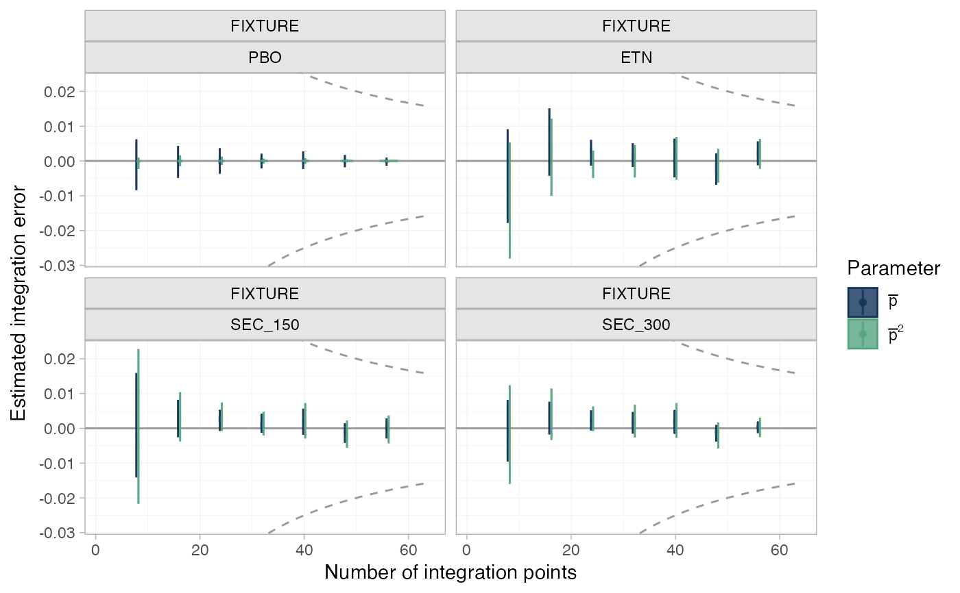
For ML-NMR models, plot the estimated numerical integration error over the entire posterior distribution, as the number of integration points increases. See (Phillippo et al. 2020; Phillippo 2019) for details.
Usage
plot_integration_error(
  x,
  ...,
  stat = "violin",
  orientation = c("vertical", "horizontal", "x", "y"),
  show_expected_rate = TRUE
)
Arguments
- x
An object of type
stan_mlnmr- ...
Additional arguments passed to the
ggdistplot stat.- stat
Character string specifying the
ggdistplot stat used to summarise the integration error over the posterior. Default is"violin", which is equivalent to"eye"with some cosmetic tweaks.- orientation
Whether the
ggdistgeom is drawn horizontally ("horizontal") or vertically ("vertical"), default"vertical"- show_expected_rate
Logical, show typical convergence rate \(1/N\)? Default
TRUE.
Details
The total number of integration points is set by the n_int
argument to add_integration(), and the intervals at which integration
error is estimated are set by the int_thin argument to nma(). The
typical convergence rate of Quasi-Monte Carlo integration (as used here) is
\(1/N\), which by default is displayed on the plot output.
The integration error at each thinning interval \(N_\mathrm{thin}\) is
estimated for each point in the posterior distribution by subtracting the
final estimate (using all n_int points) from the estimate using only the
first \(N_\mathrm{thin}\) points.
Note for survival models
This function is not supported for survival/time-to-event models. These do not save cumulative integration points for efficiency reasons (both time and memory).
Examples
## Plaque psoriasis ML-NMR
# Set up plaque psoriasis network combining IPD and AgD
library(dplyr)
pso_ipd <- filter(plaque_psoriasis_ipd,
                  studyc %in% c("UNCOVER-1", "UNCOVER-2", "UNCOVER-3"))

pso_agd <- filter(plaque_psoriasis_agd,
                  studyc == "FIXTURE")

head(pso_ipd)
#>      studyc      trtc_long    trtc trtn pasi75 pasi90 pasi100 age  bmi pasi_w0
#> 1 UNCOVER-1 Ixekizumab Q2W IXE_Q2W    2      0      0       0  34 32.2    18.2
#> 2 UNCOVER-1 Ixekizumab Q2W IXE_Q2W    2      1      0       0  64 41.9    23.4
#> 3 UNCOVER-1 Ixekizumab Q2W IXE_Q2W    2      1      1       0  42 26.2    12.8
#> 4 UNCOVER-1 Ixekizumab Q2W IXE_Q2W    2      0      0       0  45 52.9    36.0
#> 5 UNCOVER-1 Ixekizumab Q2W IXE_Q2W    2      1      0       0  67 22.9    20.9
#> 6 UNCOVER-1 Ixekizumab Q2W IXE_Q2W    2      1      1       1  57 22.4    18.2
#>    male bsa weight durnpso prevsys   psa
#> 1  TRUE  18   98.1     6.7    TRUE  TRUE
#> 2  TRUE  33  129.6    14.5   FALSE  TRUE
#> 3  TRUE  33   78.0    26.5    TRUE FALSE
#> 4 FALSE  50  139.9    25.0    TRUE  TRUE
#> 5 FALSE  35   54.2    11.9    TRUE FALSE
#> 6  TRUE  29   67.5    15.2    TRUE FALSE
head(pso_agd)
#>    studyc          trtc_long    trtc trtn pasi75_r pasi75_n pasi90_r pasi90_n
#> 1 FIXTURE         Etanercept     ETN    4      142      323       67      323
#> 2 FIXTURE            Placebo     PBO    1       16      324        5      324
#> 3 FIXTURE Secukinumab 150 mg SEC_150    5      219      327      137      327
#> 4 FIXTURE Secukinumab 300 mg SEC_300    6      249      323      175      323
#>   pasi100_r pasi100_n sample_size_w0 age_mean age_sd bmi_mean bmi_sd
#> 1        14       323            326     43.8   13.0     28.7    5.9
#> 2         0       324            326     44.1   12.6     27.9    6.1
#> 3        47       327            327     45.4   12.9     28.4    5.9
#> 4        78       323            327     44.5   13.2     28.4    6.4
#>   pasi_w0_mean pasi_w0_sd male bsa_mean bsa_sd weight_mean weight_sd
#> 1         23.2        9.8 71.2     33.6   18.0        84.6      20.5
#> 2         24.1       10.5 72.7     35.2   19.1        82.0      20.4
#> 3         23.7       10.5 72.2     34.5   19.4        83.6      20.8
#> 4         23.9        9.9 68.5     34.3   19.2        83.0      21.6
#>   durnpso_mean durnpso_sd prevsys  psa
#> 1         16.4       12.0    65.6 13.5
#> 2         16.6       11.6    62.6 15.0
#> 3         17.3       12.2    64.8 15.0
#> 4         15.8       12.3    63.0 15.3

pso_ipd <- pso_ipd %>%
  mutate(# Variable transformations
    bsa = bsa / 100,
    prevsys = as.numeric(prevsys),
    psa = as.numeric(psa),
    weight = weight / 10,
    durnpso = durnpso / 10,
    # Treatment classes
    trtclass = case_when(trtn == 1 ~ "Placebo",
                         trtn %in% c(2, 3, 5, 6) ~ "IL blocker",
                         trtn == 4 ~ "TNFa blocker"),
    # Check complete cases for covariates of interest
    complete = complete.cases(durnpso, prevsys, bsa, weight, psa)
  )

pso_agd <- pso_agd %>%
  mutate(
    # Variable transformations
    bsa_mean = bsa_mean / 100,
    bsa_sd = bsa_sd / 100,
    prevsys = prevsys / 100,
    psa = psa / 100,
    weight_mean = weight_mean / 10,
    weight_sd = weight_sd / 10,
    durnpso_mean = durnpso_mean / 10,
    durnpso_sd = durnpso_sd / 10,
    # Treatment classes
    trtclass = case_when(trtn == 1 ~ "Placebo",
                         trtn %in% c(2, 3, 5, 6) ~ "IL blocker",
                         trtn == 4 ~ "TNFa blocker")
  )

# Exclude small number of individuals with missing covariates
pso_ipd <- filter(pso_ipd, complete)

pso_net <- combine_network(
  set_ipd(pso_ipd,
          study = studyc,
          trt = trtc,
          r = pasi75,
          trt_class = trtclass),
  set_agd_arm(pso_agd,
              study = studyc,
              trt = trtc,
              r = pasi75_r,
              n = pasi75_n,
              trt_class = trtclass)
)

# Print network details
pso_net
#> A network with 3 IPD studies, and 1 AgD study (arm-based).
#>
#> ------------------------------------------------------------------- IPD studies ----
#>  Study     Treatment arms
#>  UNCOVER-1 3: IXE_Q2W | IXE_Q4W | PBO
#>  UNCOVER-2 4: ETN | IXE_Q2W | IXE_Q4W | PBO
#>  UNCOVER-3 4: ETN | IXE_Q2W | IXE_Q4W | PBO
#>
#>  Outcome type: binary
#> ------------------------------------------------------- AgD studies (arm-based) ----
#>  Study   Treatment arms
#>  FIXTURE 4: PBO | ETN | SEC_150 | SEC_300
#>
#>  Outcome type: count
#> ------------------------------------------------------------------------------------
#> Total number of treatments: 6, in 3 classes
#> Total number of studies: 4
#> Reference treatment is: PBO
#> Network is connected

# Add integration points to the network
pso_net <- add_integration(pso_net,
  durnpso = distr(qgamma, mean = durnpso_mean, sd = durnpso_sd),
  prevsys = distr(qbern, prob = prevsys),
  bsa = distr(qlogitnorm, mean = bsa_mean, sd = bsa_sd),
  weight = distr(qgamma, mean = weight_mean, sd = weight_sd),
  psa = distr(qbern, prob = psa),
  n_int = 64)
#> Using weighted average correlation matrix computed from IPD studies.

# \donttest{
# Fit the ML-NMR model
pso_fit <- nma(pso_net,
               trt_effects = "fixed",
               link = "probit",
               likelihood = "bernoulli2",
               regression = ~(durnpso + prevsys + bsa + weight + psa)*.trt,
               class_interactions = "common",
               prior_intercept = normal(scale = 10),
               prior_trt = normal(scale = 10),
               prior_reg = normal(scale = 10),
               init_r = 0.1,
               QR = TRUE,
               # Set the thinning factor for saving the cumulative results
               # (This also sets int_check = FALSE)
               int_thin = 8)
#> Note: Setting "PBO" as the network reference treatment.
pso_fit
#> A fixed effects ML-NMR with a bernoulli2 likelihood (probit link).
#> Regression model: ~(durnpso + prevsys + bsa + weight + psa) * .trt.
#> Centred covariates at the following overall mean values:
#>   durnpso   prevsys       bsa    weight       psa
#> 1.8134535 0.6450416 0.2909089 8.9369318 0.2147914
#> Inference for Stan model: binomial_2par.
#> 4 chains, each with iter=2000; warmup=1000; thin=1;
#> post-warmup draws per chain=1000, total post-warmup draws=4000.
#>
#>                                         mean se_mean   sd     2.5%      25%
#> beta[durnpso]                           0.04    0.00 0.06    -0.08     0.00
#> beta[prevsys]                          -0.14    0.00 0.16    -0.45    -0.25
#> beta[bsa]                              -0.08    0.01 0.45    -1.01    -0.36
#> beta[weight]                            0.04    0.00 0.03    -0.02     0.02
#> beta[psa]                              -0.07    0.00 0.17    -0.42    -0.19
#> beta[durnpso:.trtclassTNFa blocker]    -0.03    0.00 0.07    -0.18    -0.08
#> beta[durnpso:.trtclassIL blocker]      -0.01    0.00 0.07    -0.14    -0.06
#> beta[prevsys:.trtclassTNFa blocker]     0.19    0.00 0.19    -0.19     0.06
#> beta[prevsys:.trtclassIL blocker]       0.07    0.00 0.17    -0.28    -0.05
#> beta[bsa:.trtclassTNFa blocker]         0.07    0.01 0.52    -0.94    -0.29
#> beta[bsa:.trtclassIL blocker]           0.30    0.01 0.50    -0.64    -0.04
#> beta[weight:.trtclassTNFa blocker]     -0.17    0.00 0.04    -0.23    -0.19
#> beta[weight:.trtclassIL blocker]       -0.10    0.00 0.03    -0.16    -0.12
#> beta[psa:.trtclassTNFa blocker]        -0.06    0.00 0.21    -0.46    -0.20
#> beta[psa:.trtclassIL blocker]           0.00    0.00 0.19    -0.36    -0.12
#> d[ETN]                                  1.56    0.00 0.08     1.40     1.50
#> d[IXE_Q2W]                              2.96    0.00 0.09     2.79     2.90
#> d[IXE_Q4W]                              2.54    0.00 0.08     2.39     2.49
#> d[SEC_150]                              2.15    0.00 0.12     1.92     2.07
#> d[SEC_300]                              2.45    0.00 0.12     2.22     2.37
#> lp__                                -1576.42    0.08 3.43 -1583.89 -1578.69
#>                                          50%      75%    97.5% n_eff Rhat
#> beta[durnpso]                           0.04     0.09     0.16  5670    1
#> beta[prevsys]                          -0.14    -0.03     0.19  5527    1
#> beta[bsa]                              -0.07     0.23     0.77  5051    1
#> beta[weight]                            0.04     0.06     0.10  5746    1
#> beta[psa]                              -0.07     0.04     0.26  5391    1
#> beta[durnpso:.trtclassTNFa blocker]    -0.03     0.02     0.12  6178    1
#> beta[durnpso:.trtclassIL blocker]      -0.01     0.03     0.13  7052    1
#> beta[prevsys:.trtclassTNFa blocker]     0.19     0.31     0.56  5580    1
#> beta[prevsys:.trtclassIL blocker]       0.07     0.18     0.40  6257    1
#> beta[bsa:.trtclassTNFa blocker]         0.05     0.41     1.13  5498    1
#> beta[bsa:.trtclassIL blocker]           0.29     0.64     1.29  6710    1
#> beta[weight:.trtclassTNFa blocker]     -0.17    -0.14    -0.10  6769    1
#> beta[weight:.trtclassIL blocker]       -0.10    -0.08    -0.04  6777    1
#> beta[psa:.trtclassTNFa blocker]        -0.06     0.08     0.35  4954    1
#> beta[psa:.trtclassIL blocker]           0.00     0.13     0.38  5800    1
#> d[ETN]                                  1.55     1.61     1.71  4360    1
#> d[IXE_Q2W]                              2.96     3.02     3.12  4868    1
#> d[IXE_Q4W]                              2.54     2.60     2.70  4973    1
#> d[SEC_150]                              2.15     2.23     2.37  4897    1
#> d[SEC_300]                              2.45     2.53     2.69  5543    1
#> lp__                                -1576.06 -1573.90 -1570.67  1681    1
#>
#> Samples were drawn using NUTS(diag_e) at Fri Jun 26 12:29:52 2026.
#> For each parameter, n_eff is a crude measure of effective sample size,
#> and Rhat is the potential scale reduction factor on split chains (at
#> convergence, Rhat=1).

# Plot numerical integration error
plot_integration_error(pso_fit)

# }
# }