The plot method for nma_summary objects is used to produce plots of
parameter estimates (when called on a stan_nma object or its summary),
relative effects (when called on the output of relative_effects()),
absolute predictions (when called on the output of predict.stan_nma()),
posterior ranks and rank probabilities (when called on the output of
posterior_ranks() or posterior_rank_probs()).
Usage
# S3 method for class 'nma_summary'
plot(
  x,
  ...,
  stat = "pointinterval",
  orientation = c("horizontal", "vertical", "y", "x"),
  ref_line = NA_real_
)

# S3 method for class 'nma_parameter_summary'
plot(
  x,
  ...,
  stat = "pointinterval",
  orientation = c("horizontal", "vertical", "y", "x"),
  ref_line = NA_real_
)

# S3 method for class 'nma_rank_probs'
plot(x, ...)

# S3 method for class 'surv_nma_summary'
plot(x, ..., stat = "lineribbon")
Arguments
- x
A
nma_summaryobject- ...
Additional arguments passed on to the underlying
ggdistplot stat, see Details- stat
Character string specifying the
ggdistplot stat to use, default"pointinterval", except when plotting estimated survival/hazard/cumulative hazard curves from survival models where the default is"lineribbon"- orientation
Whether the
ggdistgeom is drawn horizontally ("horizontal") or vertically ("vertical"), default"horizontal"- ref_line
Numeric vector of positions for reference lines, by default no reference lines are drawn
Details
Plotting is handled by ggplot2 and
the stats and geoms provided in the ggdist
package. As a result, the output is very flexible. Any plotting stats
provided by ggdist may be used, via the argument stat.
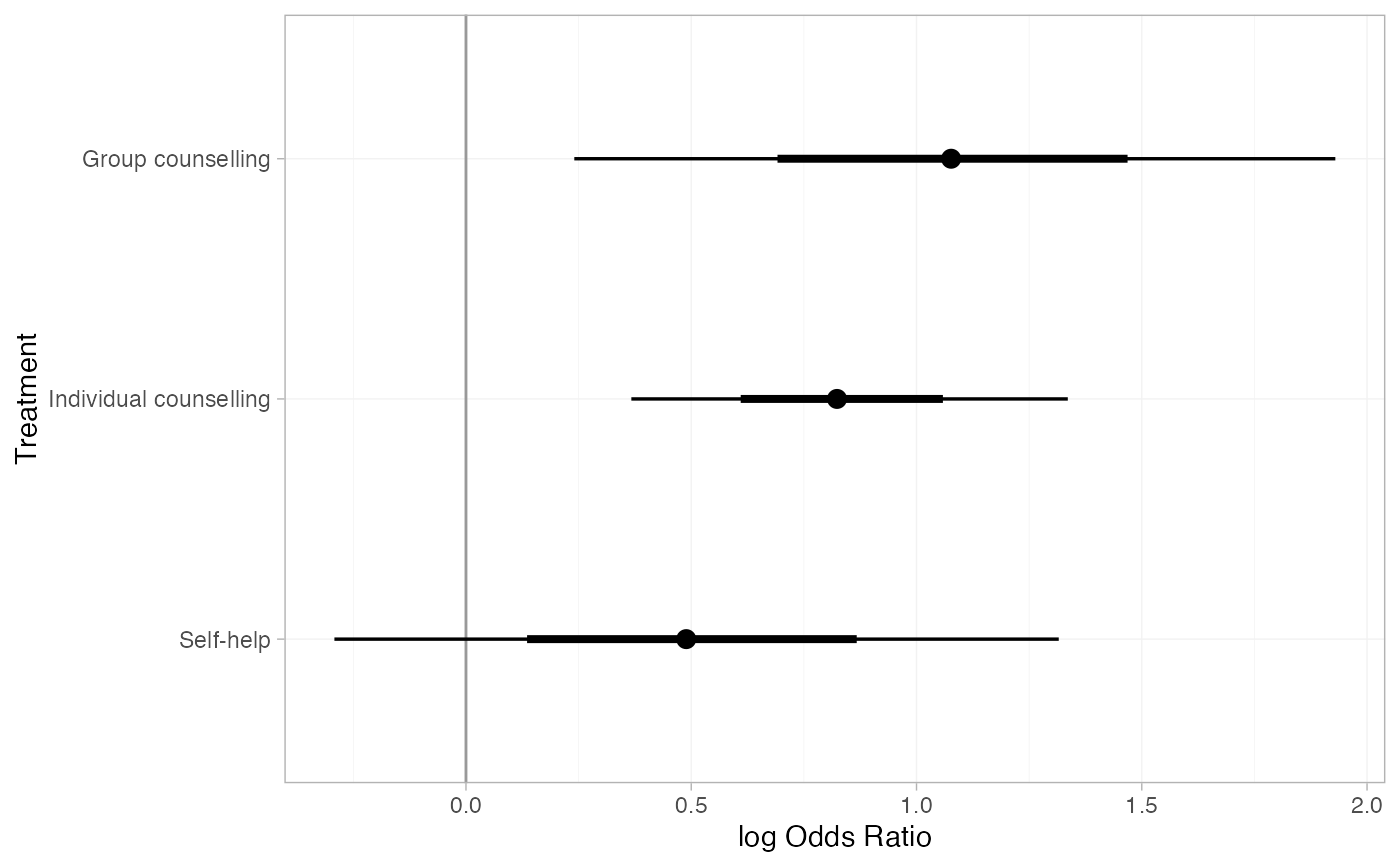
The default uses
ggdist::stat_pointinterval(), to
produce medians and 95% Credible Intervals with 66% inner bands. Additional
arguments in ... are passed to the ggdist stat, to customise the
output. For example, to produce means and Credible Intervals, specify
point_interval = "mean_qi". To produce an 80% Credible Interval with no
inner band, specify .width = c(0, 0.8).
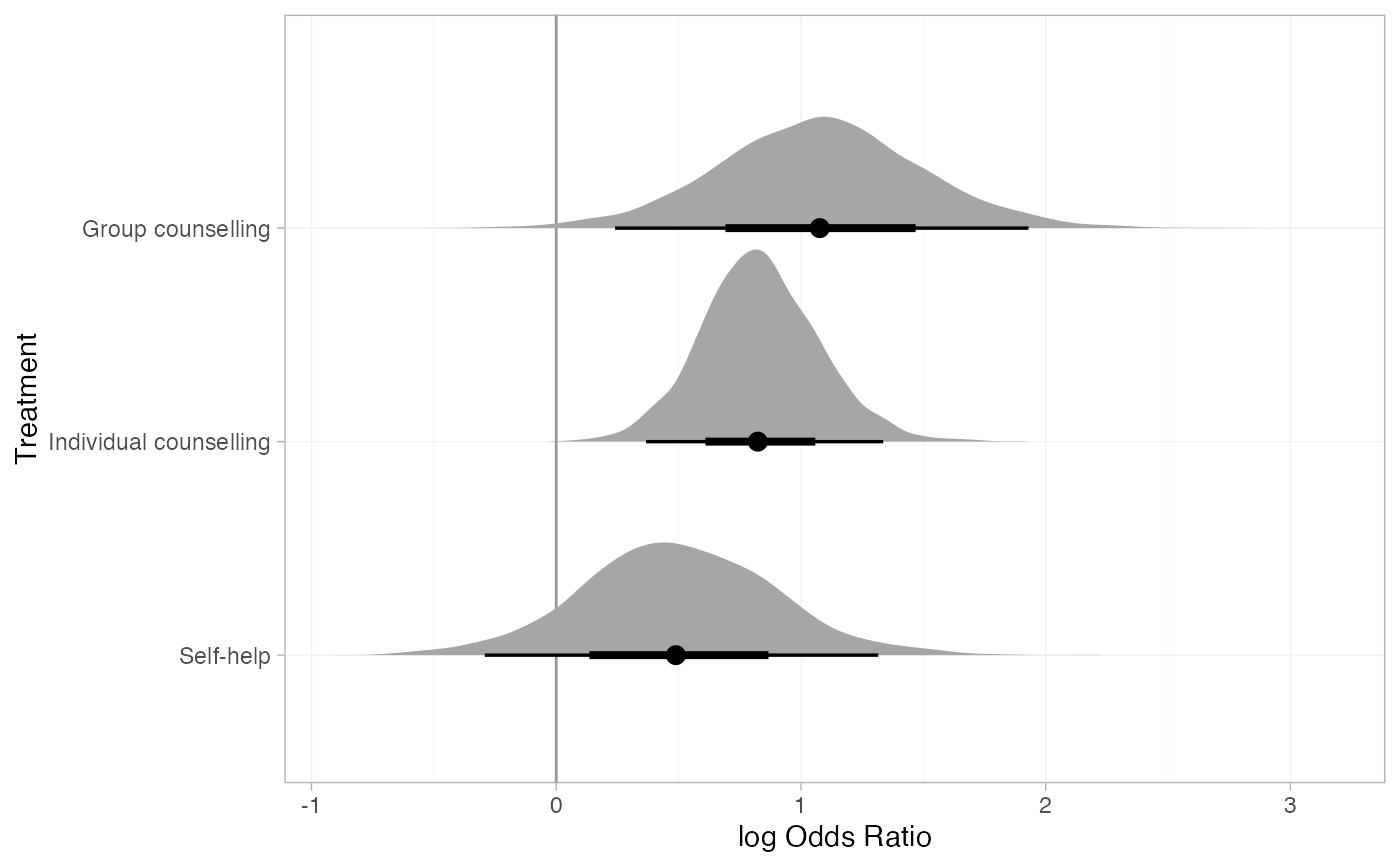
Alternative stats can be specified to produce different summaries. For
example, specify stat = "[half]eye" to produce (half) eye plots, or stat = "histinterval" to produce histograms with intervals.
A full list of options and examples is found in the ggdist vignette
vignette("slabinterval", package = "ggdist").
For survival/hazard/cumulative hazard curves estimated from survival
models, the default uses
ggdist::stat_lineribbon() which
produces curves of posterior medians with 50%, 80%, and 95% Credible
Interval bands. Again, additional arguments in ... are passed to the
ggdist stat. For example, to produce posterior means and 95% Credible
bands, specify point_interval = "mean_qi" and .width = 0.95.
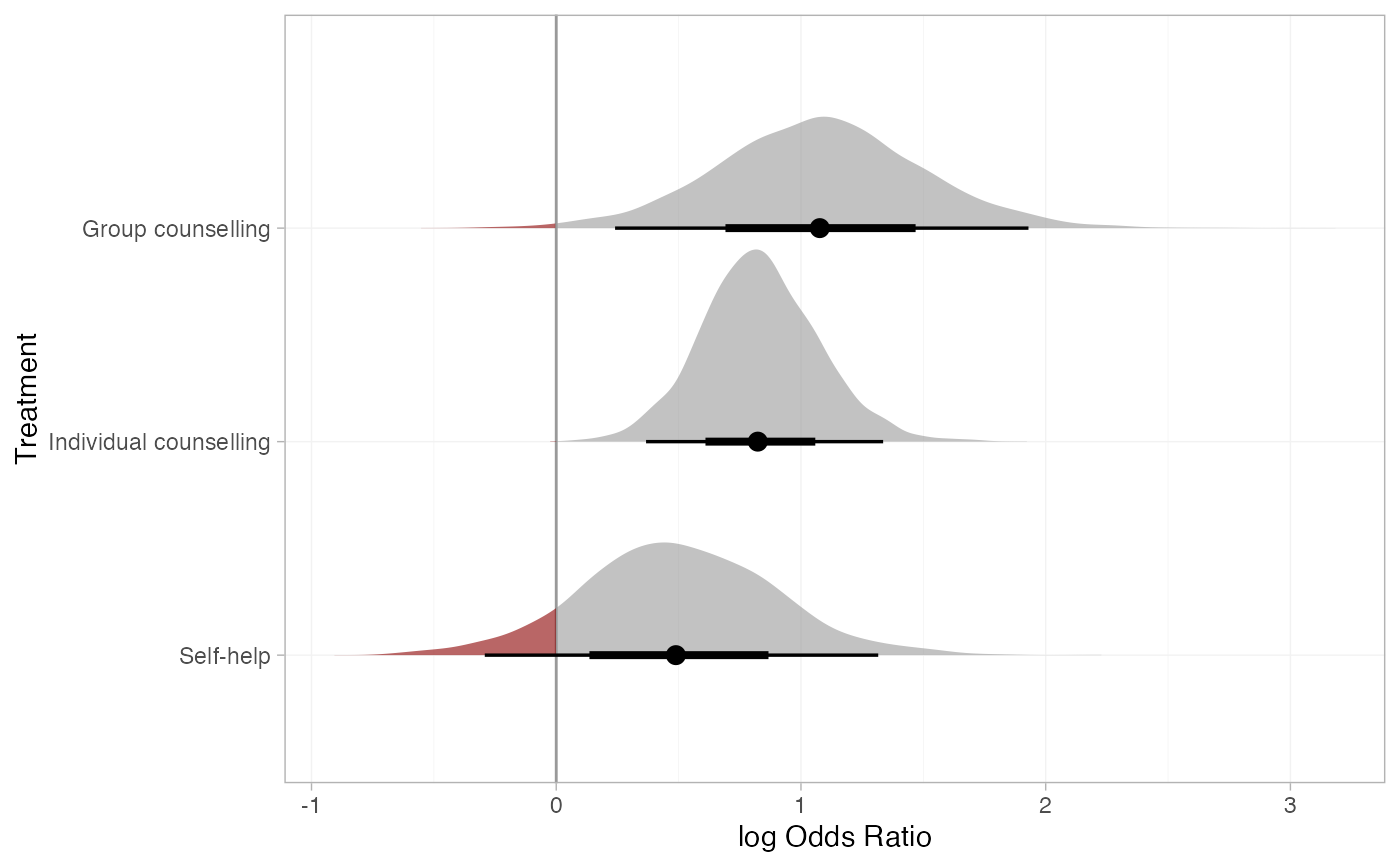
A ggplot object is returned which can be further modified through the
usual ggplot2 functions to add further
aesthetics, geoms, themes, etc.
Examples
## Smoking cessation
# \donttest{
# Run smoking RE NMA example if not already available
if (!exists("smk_fit_RE")) example("example_smk_re", run.donttest = TRUE)
# }
# \donttest{
# Produce relative effects
smk_releff_RE <- relative_effects(smk_fit_RE)
plot(smk_releff_RE, ref_line = 0)
 # Customise plot options
plot(smk_releff_RE, ref_line = 0, stat = "halfeye")
 # Further customisation is possible with ggplot commands
plot(smk_releff_RE, ref_line = 0, stat = "halfeye", slab_alpha = 0.6) +
ggplot2::aes(slab_fill = ggplot2::after_stat(ifelse(x < 0, "darkred", "grey60")))
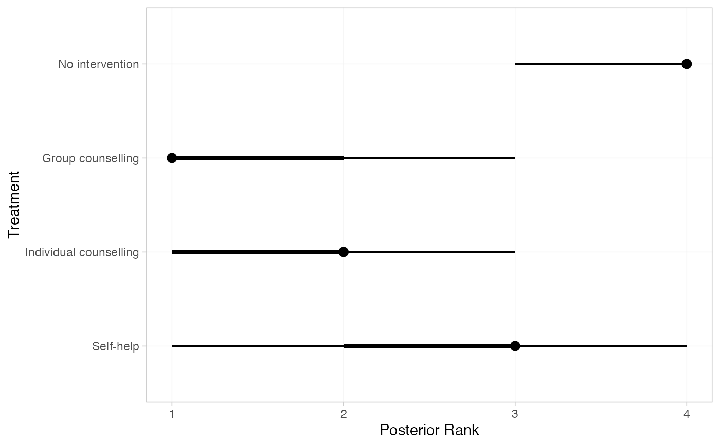
 # Produce posterior ranks
smk_rank_RE <- posterior_ranks(smk_fit_RE, lower_better = FALSE)
plot(smk_rank_RE)
 # Produce rank probabilities
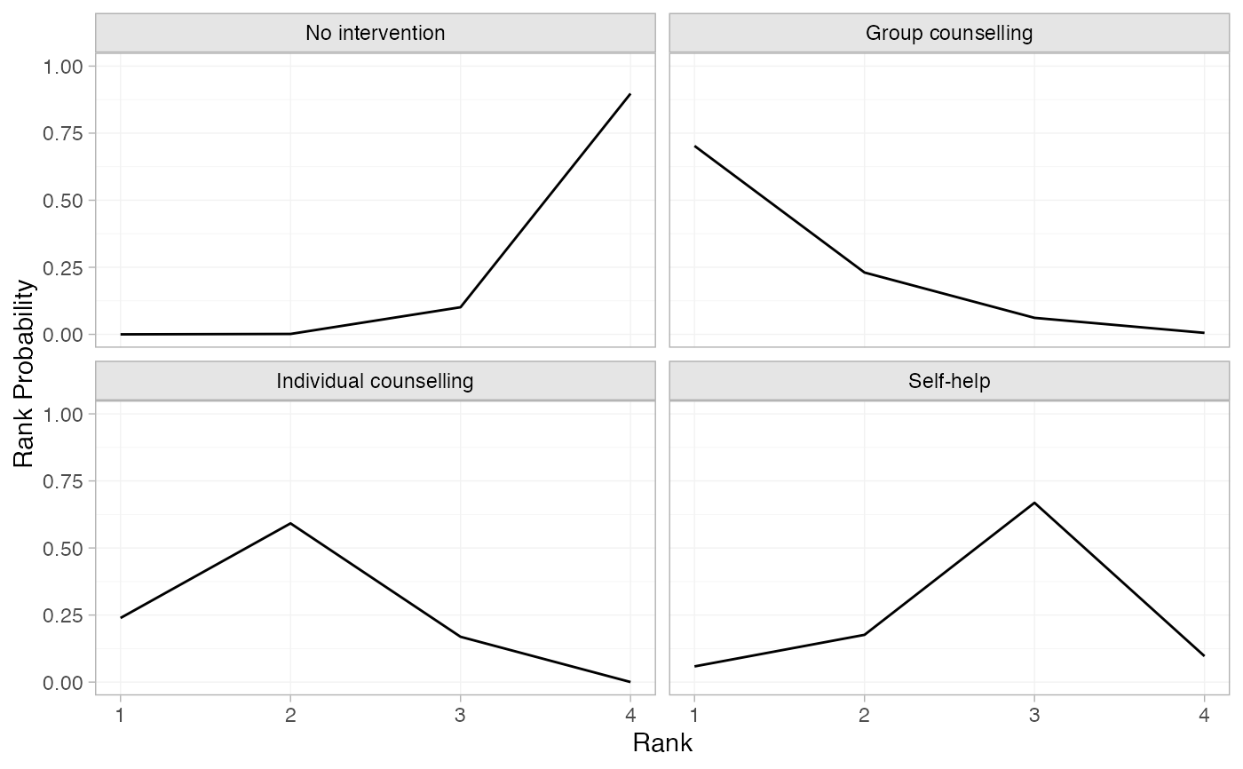
smk_rankprob_RE <- posterior_rank_probs(smk_fit_RE, lower_better = FALSE)
plot(smk_rankprob_RE)
 # Produce cumulative rank probabilities
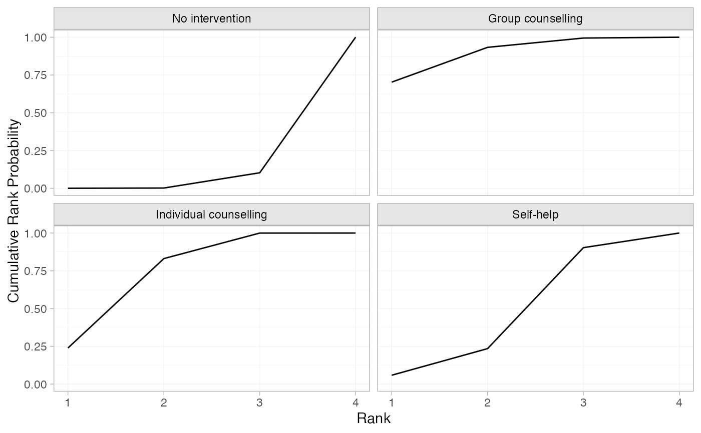
smk_cumrankprob_RE <- posterior_rank_probs(smk_fit_RE, lower_better = FALSE,
cumulative = TRUE)
plot(smk_cumrankprob_RE)
 # Further customisation is possible with ggplot commands
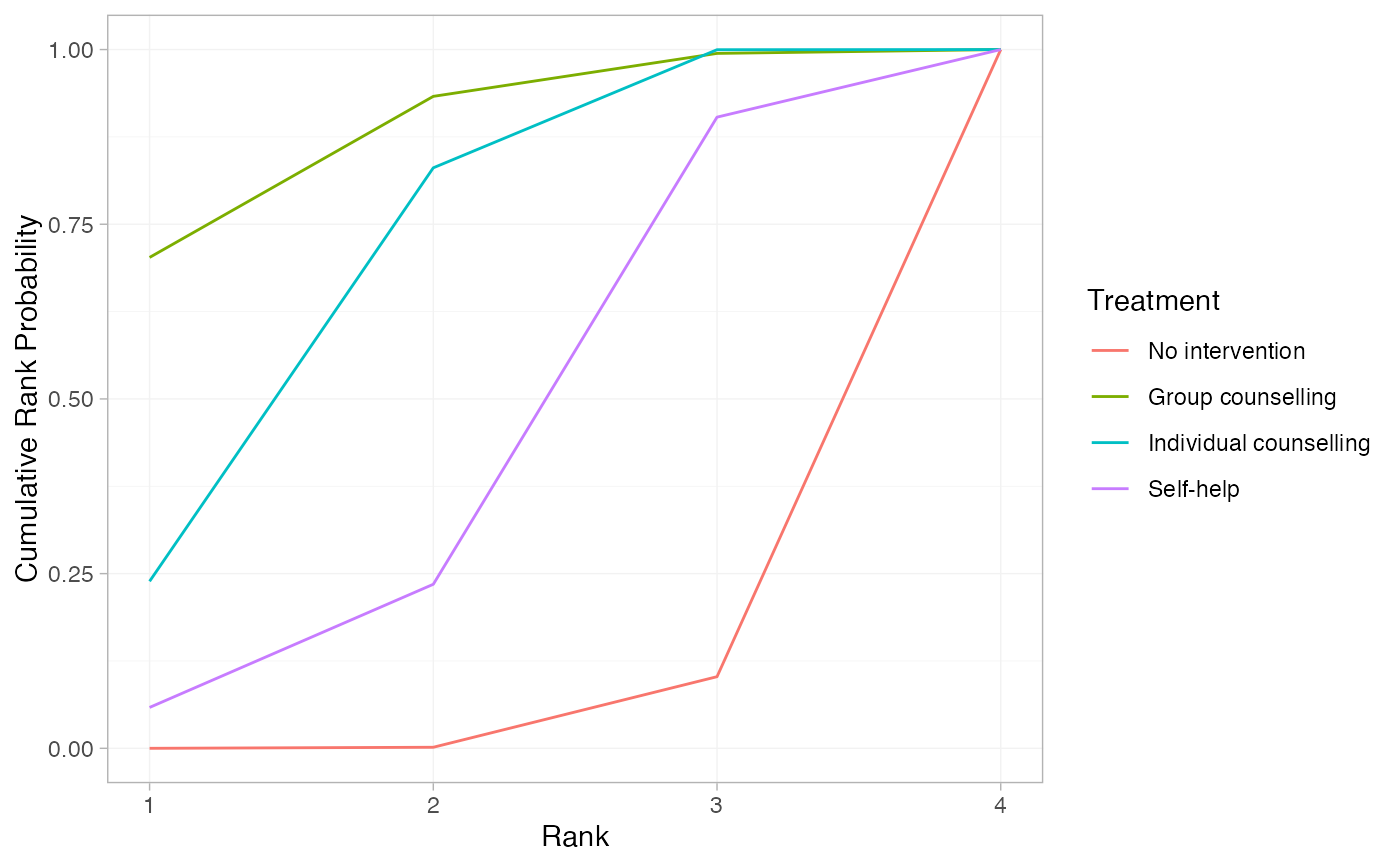
plot(smk_cumrankprob_RE) +
ggplot2::facet_null() +
ggplot2::aes(colour = Treatment)
 # }
# }