library(multinma)
options(mc.cores = parallel::detectCores())
#> For execution on a local, multicore CPU with excess RAM we recommend calling
#> options(mc.cores = parallel::detectCores())
#>
#> Attaching package: 'multinma'
#> The following objects are masked from 'package:stats':
#>
#> dgamma, pgamma, qgammaThis vignette describes the analysis of 10 trials comparing reduced
fat diets to control (non-reduced fat diets) for preventing mortality
(Hooper et al.
2000; Dias et al. 2011). The data are
available in this package as dietary_fat:
head(dietary_fat)
#>   studyn            studyc trtn        trtc   r    n      E
#> 1      1              DART    1     Control 113 1015 1917.0
#> 2      1              DART    2 Reduced Fat 111 1018 1925.0
#> 3      2 London Corn/Olive    1     Control   1   26   43.6
#> 4      2 London Corn/Olive    2 Reduced Fat   5   28   41.3
#> 5      2 London Corn/Olive    2 Reduced Fat   3   26   38.0
#> 6      3    London Low Fat    1     Control  24  129  393.5
Setting up the network
We begin by setting up the network - here just a pairwise
meta-analysis. We have arm-level rate data giving the number of deaths
(r) and the person-years at risk (E) in each
arm, so we use the function set_agd_arm(). We set “Control”
as the reference treatment.
diet_net <- set_agd_arm(dietary_fat,
                        study = studyc,
                        trt = trtc,
                        r = r,
                        E = E,
                        trt_ref = "Control",
                        sample_size = n)
diet_net
#> A network with 10 AgD studies (arm-based).
#>
#> ------------------------------------------------------- AgD studies (arm-based) ----
#>  Study                   Treatment arms
#>  DART                    2: Control | Reduced Fat
#>  London Corn/Olive       3: Control | Reduced Fat | Reduced Fat
#>  London Low Fat          2: Control | Reduced Fat
#>  Minnesota Coronary      2: Control | Reduced Fat
#>  MRC Soya                2: Control | Reduced Fat
#>  Oslo Diet-Heart         2: Control | Reduced Fat
#>  STARS                   2: Control | Reduced Fat
#>  Sydney Diet-Heart       2: Control | Reduced Fat
#>  Veterans Administration 2: Control | Reduced Fat
#>  Veterans Diet & Skin CA 2: Control | Reduced Fat
#>
#>  Outcome type: rate
#> ------------------------------------------------------------------------------------
#> Total number of treatments: 2
#> Total number of studies: 10
#> Reference treatment is: Control
#> Network is connected
We also specify the optional sample_size argument,
although it is not strictly necessary here. In this case
sample_size would only be required to produce a network
plot with nodes weighted by sample size, and a network plot is not
particularly informative for a meta-analysis of only two treatments.
(The sample_size argument is more important when a
regression model is specified, since it also enables automatic centering
of predictors and production of predictions for studies in the network,
see ?set_agd_arm.)
Meta-analysis models
We fit both fixed effect (FE) and random effects (RE) models.
Fixed effect meta-analysis
First, we fit a fixed effect model using the nma()
function with trt_effects = "fixed". We use \mathrm{N}(0, 100^2) prior distributions for
the treatment effects d_k and
study-specific intercepts \mu_j. We can
examine the range of parameter values implied by these prior
distributions with the summary() method:
summary(normal(scale = 100))
#> A Normal prior distribution: location = 0, scale = 100.
#> 50% of the prior density lies between -67.45 and 67.45.
#> 95% of the prior density lies between -196 and 196.
The model is fitted using the nma() function. By
default, this will use a Poisson likelihood with a log link function,
auto-detected from the data.
diet_fit_FE <- nma(diet_net,
                   trt_effects = "fixed",
                   prior_intercept = normal(scale = 100),
                   prior_trt = normal(scale = 100))
Basic parameter summaries are given by the print()
method:
diet_fit_FE
#> A fixed effects NMA with a poisson likelihood (log link).
#> Inference for Stan model: poisson.
#> 4 chains, each with iter=2000; warmup=1000; thin=1;
#> post-warmup draws per chain=1000, total post-warmup draws=4000.
#>
#>                   mean se_mean   sd    2.5%     25%     50%     75%   97.5% n_eff Rhat
#> d[Reduced Fat]   -0.01    0.00 0.05   -0.11   -0.04   -0.01    0.03    0.10  3568    1
#> lp__           5386.16    0.06 2.49 5380.38 5384.77 5386.50 5387.97 5389.91  1586    1
#>
#> Samples were drawn using NUTS(diag_e) at Fri Apr 17 08:34:59 2026.
#> For each parameter, n_eff is a crude measure of effective sample size,
#> and Rhat is the potential scale reduction factor on split chains (at
#> convergence, Rhat=1).
By default, summaries of the study-specific intercepts \mu_j are hidden, but could be examined by
changing the pars argument:
The prior and posterior distributions can be compared visually using
the plot_prior_posterior() function:
plot_prior_posterior(diet_fit_FE)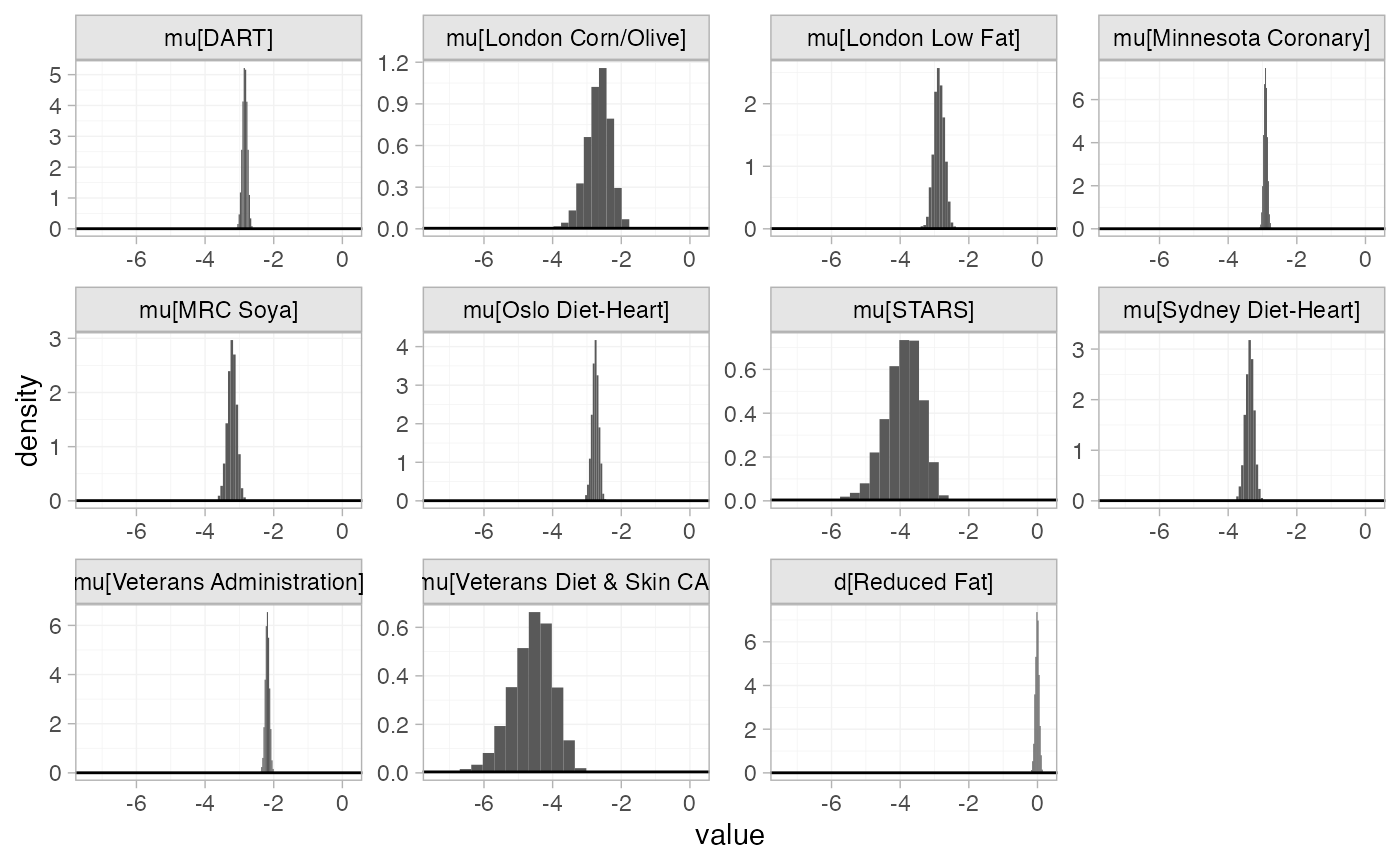
Random effects meta-analysis
We now fit a random effects model using the nma()
function with trt_effects = "random". Again, we use \mathrm{N}(0, 100^2) prior distributions for
the treatment effects d_k and
study-specific intercepts \mu_j, and we
additionally use a \textrm{half-N}(5^2)
prior for the heterogeneity standard deviation \tau. We can examine the range of parameter
values implied by these prior distributions with the
summary() method:
summary(normal(scale = 100))
#> A Normal prior distribution: location = 0, scale = 100.
#> 50% of the prior density lies between -67.45 and 67.45.
#> 95% of the prior density lies between -196 and 196.
summary(half_normal(scale = 5))
#> A half-Normal prior distribution: scale = 5.
#> 50% of the prior density lies between 0 and 3.37.
#> 95% of the prior density lies between 0 and 9.8.
Fitting the RE model
diet_fit_RE <- nma(diet_net,
                   trt_effects = "random",
                   prior_intercept = normal(scale = 100),
                   prior_trt = normal(scale = 100),
                   prior_het = half_normal(scale = 5))
Basic parameter summaries are given by the print()
method:
diet_fit_RE
#> A random effects NMA with a poisson likelihood (log link).
#> Inference for Stan model: poisson.
#> 4 chains, each with iter=2000; warmup=1000; thin=1;
#> post-warmup draws per chain=1000, total post-warmup draws=4000.
#>
#>                   mean se_mean   sd    2.5%     25%     50%     75%   97.5% n_eff Rhat
#> d[Reduced Fat]   -0.02    0.00 0.09   -0.19   -0.06   -0.02    0.03    0.15  1581    1
#> lp__           5379.23    0.11 3.74 5371.41 5376.76 5379.38 5381.88 5385.92  1217    1
#> tau               0.13    0.00 0.12    0.01    0.05    0.10    0.18    0.45   819    1
#>
#> Samples were drawn using NUTS(diag_e) at Fri Apr 17 08:35:06 2026.
#> For each parameter, n_eff is a crude measure of effective sample size,
#> and Rhat is the potential scale reduction factor on split chains (at
#> convergence, Rhat=1).
By default, summaries of the study-specific intercepts \mu_j and study-specific relative effects
\delta_{jk} are hidden, but could be
examined by changing the pars argument:
The prior and posterior distributions can be compared visually using
the plot_prior_posterior() function:
plot_prior_posterior(diet_fit_RE, prior = c("trt", "het"))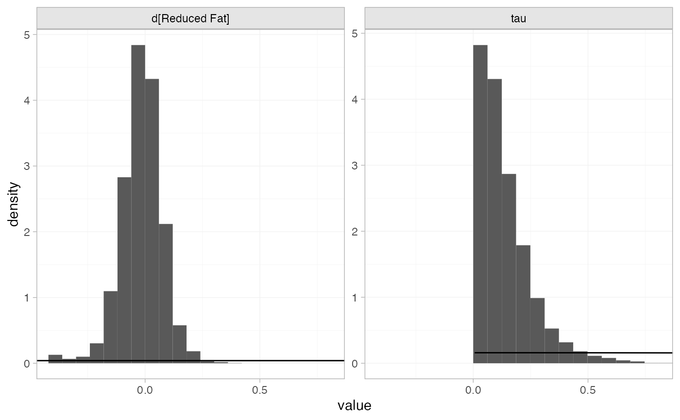
Model comparison
Model fit can be checked using the dic() function:
(dic_FE <- dic(diet_fit_FE))
#> Residual deviance: 22.5 (on 21 data points)
#>                pD: 11.3
#>               DIC: 33.8
(dic_RE <- dic(diet_fit_RE))
#> Residual deviance: 21.4 (on 21 data points)
#>                pD: 13.5
#>               DIC: 34.9
Both models appear to fit the data well, as the residual deviance is close to the number of data points. The DIC is very similar between models, so the FE model may be preferred for parsimony.
We can also examine the residual deviance contributions with the
corresponding plot() method.
plot(dic_FE)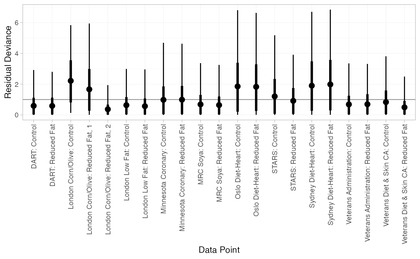
plot(dic_RE)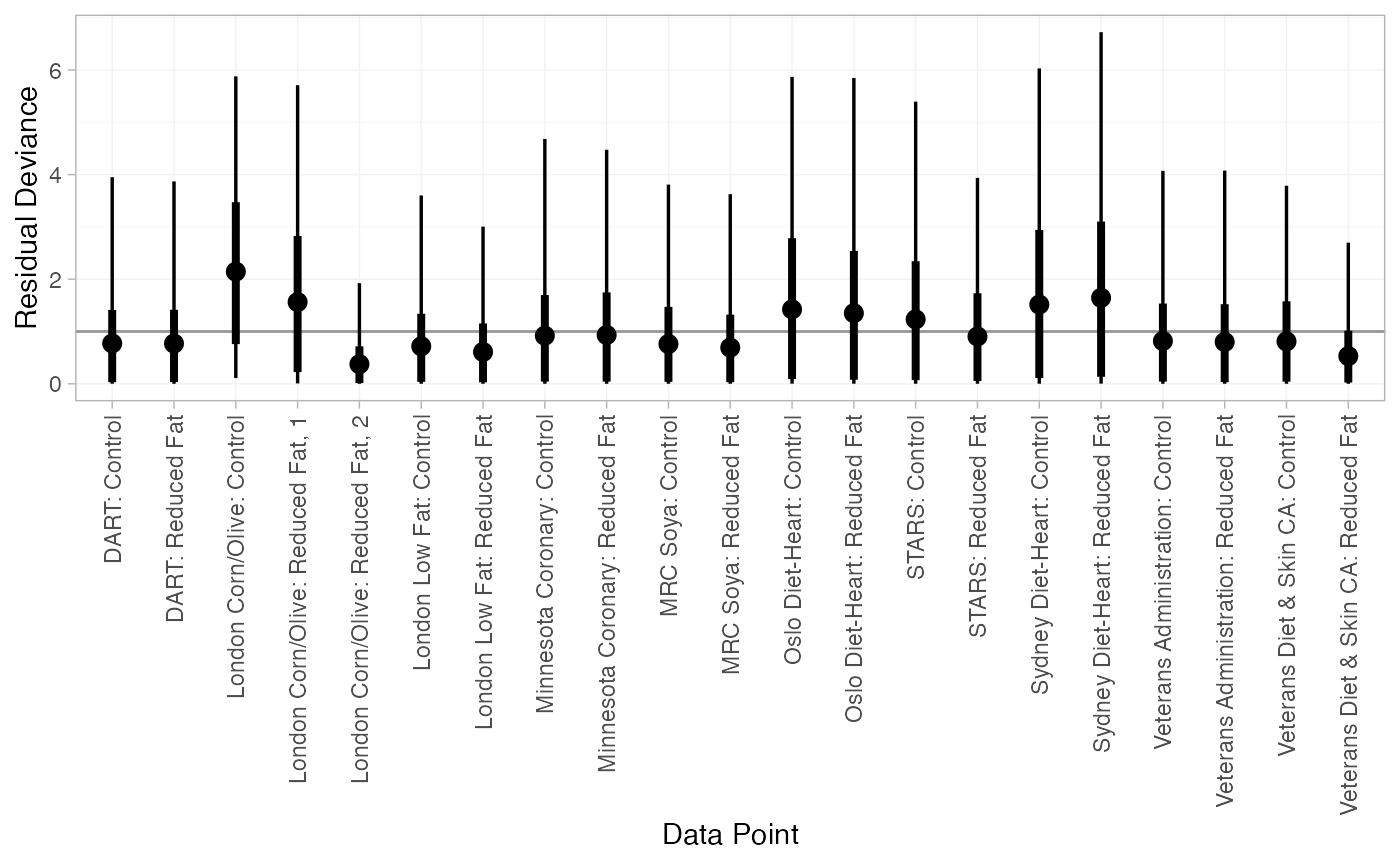
Further results
Dias et al. (2011) produce absolute predictions of the
mortality rates on reduced fat and control diets, assuming a Normal
distribution on the baseline log rate of mortality with mean -3 and precision 1.77. We can replicate these results using
the predict() method. The baseline argument
takes a distr() distribution object, with which we specify
the corresponding Normal distribution. We set
type = "response" to produce predicted rates
(type = "link" would produce predicted log rates).
pred_FE <- predict(diet_fit_FE,
                   baseline = distr(qnorm, mean = -3, sd = 1.77^-0.5),
                   type = "response")
pred_FE
#>                   mean   sd 2.5%  25%  50%  75% 97.5% Bulk_ESS Tail_ESS Rhat
#> pred[Control]     0.06 0.05 0.01 0.03 0.05 0.08  0.21     4142     3904    1
#> pred[Reduced Fat] 0.06 0.05 0.01 0.03 0.05 0.08  0.21     4118     3909    1
plot(pred_FE)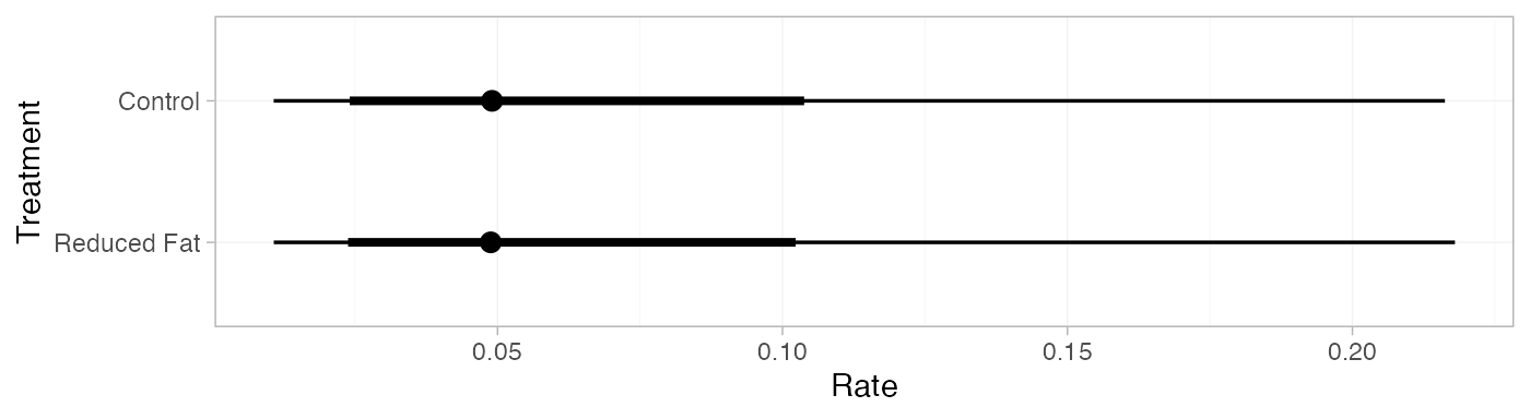
pred_RE <- predict(diet_fit_RE,
                   baseline = distr(qnorm, mean = -3, sd = 1.77^-0.5),
                   type = "response")
pred_RE
#>                   mean   sd 2.5%  25%  50%  75% 97.5% Bulk_ESS Tail_ESS Rhat
#> pred[Control]     0.07 0.06 0.01 0.03 0.05 0.08  0.22     4379     3576    1
#> pred[Reduced Fat] 0.07 0.06 0.01 0.03 0.05 0.08  0.21     4394     3531    1
plot(pred_RE)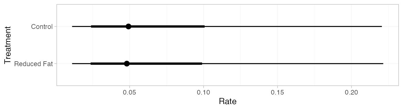
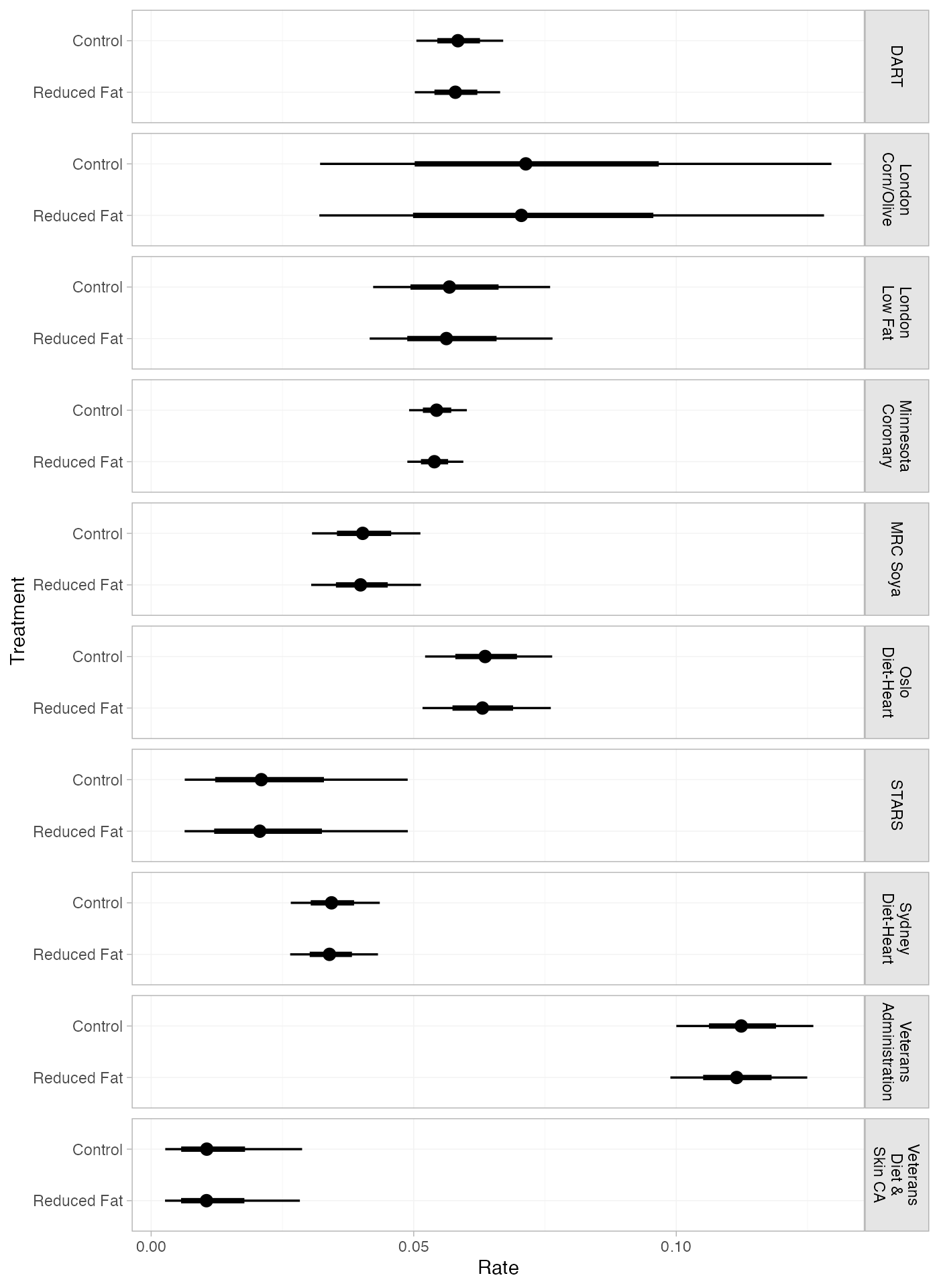
If the baseline argument is omitted, predicted rates
will be produced for every study in the network based on their estimated
baseline log rate \mu_j:
pred_FE_studies <- predict(diet_fit_FE, type = "response")
pred_FE_studies
#> ------------------------------------------------------------------- Study: DART ----
#>
#>                         mean sd 2.5%  25%  50%  75% 97.5% Bulk_ESS Tail_ESS Rhat
#> pred[DART: Control]     0.06  0 0.05 0.06 0.06 0.06  0.07     6187     3190    1
#> pred[DART: Reduced Fat] 0.06  0 0.05 0.06 0.06 0.06  0.07     7818     3376    1
#>
#> ------------------------------------------------------ Study: London Corn/Olive ----
#>
#>                                      mean   sd 2.5%  25%  50%  75% 97.5% Bulk_ESS Tail_ESS
#> pred[London Corn/Olive: Control]     0.07 0.03 0.03 0.06 0.07 0.09  0.13     8422     3035
#> pred[London Corn/Olive: Reduced Fat] 0.07 0.02 0.03 0.06 0.07 0.09  0.13     8512     3110
#>                                      Rhat
#> pred[London Corn/Olive: Control]        1
#> pred[London Corn/Olive: Reduced Fat]    1
#>
#> --------------------------------------------------------- Study: London Low Fat ----
#>
#>                                   mean   sd 2.5%  25%  50%  75% 97.5% Bulk_ESS Tail_ESS Rhat
#> pred[London Low Fat: Control]     0.06 0.01 0.04 0.05 0.06 0.06  0.08     7697     2749    1
#> pred[London Low Fat: Reduced Fat] 0.06 0.01 0.04 0.05 0.06 0.06  0.08     8588     2715    1
#>
#> ----------------------------------------------------- Study: Minnesota Coronary ----
#>
#>                                       mean sd 2.5%  25%  50%  75% 97.5% Bulk_ESS Tail_ESS Rhat
#> pred[Minnesota Coronary: Control]     0.05  0 0.05 0.05 0.05 0.06  0.06     5035     3586    1
#> pred[Minnesota Coronary: Reduced Fat] 0.05  0 0.05 0.05 0.05 0.06  0.06     6263     3698    1
#>
#> --------------------------------------------------------------- Study: MRC Soya ----
#>
#>                             mean   sd 2.5%  25%  50%  75% 97.5% Bulk_ESS Tail_ESS Rhat
#> pred[MRC Soya: Control]     0.04 0.01 0.03 0.04 0.04 0.04  0.05     7530     2448    1
#> pred[MRC Soya: Reduced Fat] 0.04 0.01 0.03 0.04 0.04 0.04  0.05     8515     2983    1
#>
#> -------------------------------------------------------- Study: Oslo Diet-Heart ----
#>
#>                                    mean   sd 2.5%  25%  50%  75% 97.5% Bulk_ESS Tail_ESS Rhat
#> pred[Oslo Diet-Heart: Control]     0.06 0.01 0.05 0.06 0.06 0.07  0.08     6664     3113    1
#> pred[Oslo Diet-Heart: Reduced Fat] 0.06 0.01 0.05 0.06 0.06 0.07  0.08     8209     3279    1
#>
#> ------------------------------------------------------------------ Study: STARS ----
#>
#>                          mean   sd 2.5%  25%  50%  75% 97.5% Bulk_ESS Tail_ESS Rhat
#> pred[STARS: Control]     0.02 0.01 0.01 0.01 0.02 0.03  0.05     6720     2887    1
#> pred[STARS: Reduced Fat] 0.02 0.01 0.01 0.01 0.02 0.03  0.05     6802     2867    1
#>
#> ------------------------------------------------------ Study: Sydney Diet-Heart ----
#>
#>                                      mean sd 2.5%  25%  50%  75% 97.5% Bulk_ESS Tail_ESS Rhat
#> pred[Sydney Diet-Heart: Control]     0.03  0 0.03 0.03 0.03 0.04  0.04     7106     2707    1
#> pred[Sydney Diet-Heart: Reduced Fat] 0.03  0 0.03 0.03 0.03 0.04  0.04     7635     2816    1
#>
#> ------------------------------------------------ Study: Veterans Administration ----
#>
#>                                            mean   sd 2.5%  25%  50%  75% 97.5% Bulk_ESS
#> pred[Veterans Administration: Control]     0.11 0.01  0.1 0.11 0.11 0.12  0.13     5091
#> pred[Veterans Administration: Reduced Fat] 0.11 0.01  0.1 0.11 0.11 0.12  0.12     6910
#>                                            Tail_ESS Rhat
#> pred[Veterans Administration: Control]         3139    1
#> pred[Veterans Administration: Reduced Fat]     3250    1
#>
#> ------------------------------------------------ Study: Veterans Diet & Skin CA ----
#>
#>                                            mean   sd 2.5%  25%  50%  75% 97.5% Bulk_ESS
#> pred[Veterans Diet & Skin CA: Control]     0.01 0.01    0 0.01 0.01 0.02  0.03     5371
#> pred[Veterans Diet & Skin CA: Reduced Fat] 0.01 0.01    0 0.01 0.01 0.02  0.03     5342
#>                                            Tail_ESS Rhat
#> pred[Veterans Diet & Skin CA: Control]         2466    1
#> pred[Veterans Diet & Skin CA: Reduced Fat]     2556    1
plot(pred_FE_studies) + ggplot2::facet_grid(Study~., labeller = ggplot2::label_wrap_gen(width = 10))