Working with 3D MCMC arrays

3D MCMC arrays (Iterations, Chains, Parameters) are produced by as.array() methods applied to stan_nma or nma_summary objects.

Usage

# S3 method for mcmc_array
summary(object, ..., probs = c(0.025, 0.25, 0.5, 0.75, 0.975))

# S3 method for mcmc_array
print(x, ...)

# S3 method for mcmc_array
plot(x, ...)

# S3 method for mcmc_array
names(x)

# S3 method for mcmc_array
names(x) <- value

Arguments

...

Further arguments passed to other methods

probs

Numeric vector of quantiles of interest

x, object

A 3D MCMC array of class mcmc_array

value

Character vector of replacement parameter names

Value

The summary() method returns a nma_summary object, the print()

method returns x invisibly. The names() method returns a character vector of parameter names, and names()<- returns the object with updated parameter names. The plot() method is a shortcut for plot(summary(x), ...), passing all arguments on to plot.nma_summary().

Examples

## Smoking cessation
# \donttest{
# Run smoking RE NMA example if not already available
if (!exists("smk_fit_RE")) example("example_smk_re", run.donttest = TRUE)
# }
# \donttest{
# Working with arrays of posterior draws (as mcmc_array objects) is
# convenient when transforming parameters

# Transforming log odds ratios to odds ratios
LOR_array <- as.array(relative_effects(smk_fit_RE))
OR_array <- exp(LOR_array)

# mcmc_array objects can be summarised to produce a nma_summary object
smk_OR_RE <- summary(OR_array)

# This can then be printed or plotted
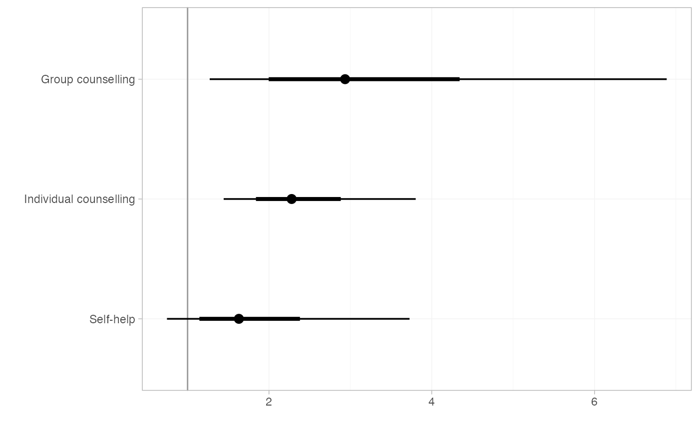
smk_OR_RE
#>                           mean   sd 2.5%  25%  50%  75% 97.5% Bulk_ESS Tail_ESS
#> d[Group counselling]      3.32 1.54 1.32 2.28 2.97 3.99  7.10     2243     2523
#> d[Individual counselling] 2.41 0.60 1.47 2.00 2.33 2.73  3.83     1190     2147
#> d[Self-help]              1.78 0.74 0.74 1.28 1.64 2.13  3.59     1897     2560
#>                           Rhat
#> d[Group counselling]         1
#> d[Individual counselling]    1
#> d[Self-help]                 1
plot(smk_OR_RE, ref_line = 1)


# Transforming heterogeneity SD to variance
tau_array <- as.array(smk_fit_RE, pars = "tau")
tausq_array <- tau_array^2

# Correct parameter names
names(tausq_array) <- "tausq"

# Summarise
summary(tausq_array)
#>       mean   sd 2.5%  25%  50%  75% 97.5% Bulk_ESS Tail_ESS Rhat
#> tausq 0.72 0.33 0.29 0.49 0.65 0.87  1.52     1286     1830    1
# }