The plot() method for nma_dic objects produced by dic() produces
several useful diagnostic plots for checking model fit and model comparison.
Further detail on these plots and their interpretation is given by
Dias et al. (2011)
.
Arguments
- x
A
nma_dicobject- y
(Optional) A second
nma_dicobject, to produce "dev-dev" plots for model comparison.- ...
Additional arguments passed on to other methods
- type
With a single
nma_dicobject, whether to show the residual deviance contribution for each data point ("resdev", the default), or a leverage plot ("leverage").- show_uncertainty
Logical, show uncertainty with a
ggdistplot stat? DefaultTRUE. Ignored fortype = "leverage".- stat
Character string specifying the
ggdistplot stat to use ifshow_uncertainty = TRUE, default"pointinterval". Ifyis provided, currently only"pointinterval"is supported.- orientation
Whether the
ggdistgeom is drawn horizontally ("horizontal") or vertically ("vertical"). Only used for residual deviance plots, default"vertical".- dic_contours
Numeric vector of DIC contribution contours to show on leverage plots, default
1:4.
Details
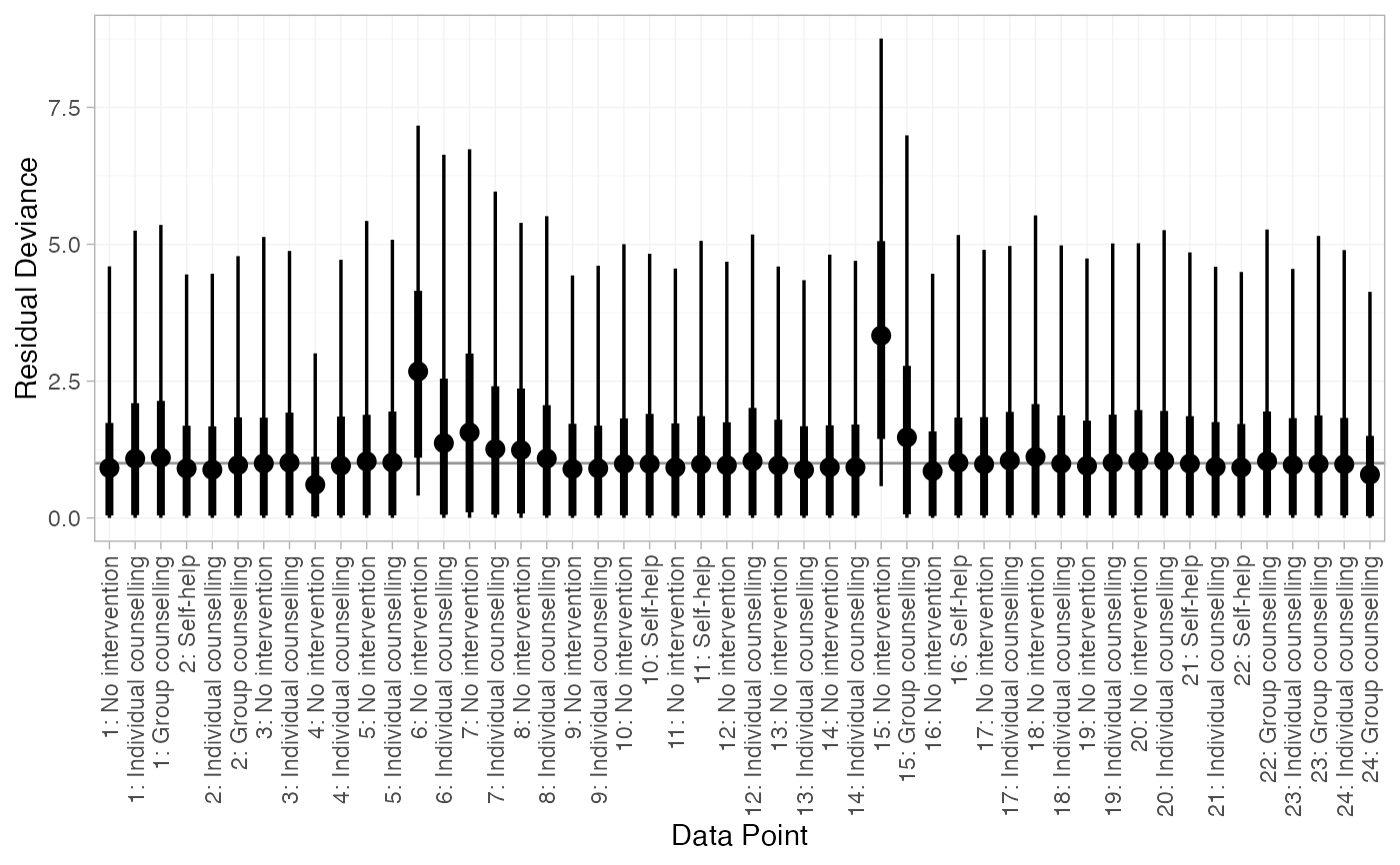
When a single nma_dic object is given, the default plot (type = "resdev") shows the residual deviance contribution for each data point.
For a good fitting model, each data point is expected to have a residual
deviance equal to its degrees of freedom (typically 1, except for multi-arm
trials in contrast format or multinomial outcomes); larger values indicate
data points that are fit poorly by the model. A leverage plot can be
produced with type = "leverage", plotting the leverages (contributions to
\(p_D\)) against the signed square root residual deviance, both
standardised by the degrees of freedom. Contours for different DIC
contribution cutoffs are also shown; points which lie outside the DIC=3
contour are generally identified as contributing to a model's poor fit.
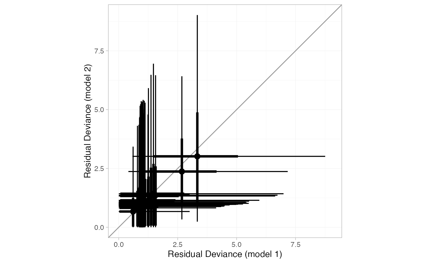
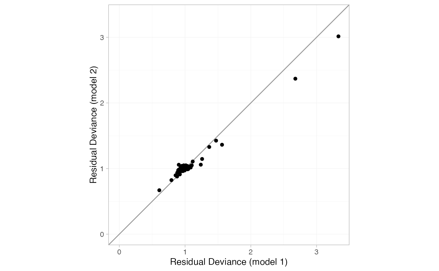
When two nma_dic objects are given, a "dev-dev" plot comparing the
residual deviance contributions under each model is produced. Data points
with residual deviance contributions lying on the line of equality are fit
equally well under either model. Data points lying below the line of
equality indicate better fit under the second model (y); conversely, data
points lying above the line of equality indicate better fit under the first
model (x). A common use case is to compare a standard consistency model
(fitted using nma() with consistency = "consistency") with an unrelated
mean effects (UME) inconsistency model (fitted using nma() with
consistency = "ume"), to check for potential inconsistency.
See Dias et al. (2011) for further details.
References
Dias S, Welton NJ, Sutton AJ, Ades AE (2011). “NICE DSU Technical Support Document 2: A generalised linear modelling framework for pair-wise and network meta-analysis of randomised controlled trials.” National Institute for Health and Care Excellence. https://sheffield.ac.uk/nice-dsu.
Examples
## Smoking cessation
# \donttest{
# Run smoking FE NMA example if not already available
if (!exists("smk_fit_FE")) example("example_smk_fe", run.donttest = TRUE)
# }
# \donttest{
# Run smoking RE NMA example if not already available
if (!exists("smk_fit_RE")) example("example_smk_re", run.donttest = TRUE)
# }
# \donttest{
# Compare DIC of FE and RE models
(smk_dic_FE <- dic(smk_fit_FE))
#> Residual deviance: 267.1 (on 50 data points)
#> pD: 26.9
#> DIC: 293.9
(smk_dic_RE <- dic(smk_fit_RE)) # substantially better fit
#> Residual deviance: 54.5 (on 50 data points)
#> pD: 44
#> DIC: 98.4
# Plot residual deviance contributions under RE model
plot(smk_dic_RE)
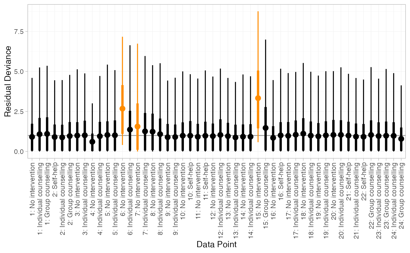
 # Further customisation is possible using ggplot commands
# For example, highlighting data points with residual deviance above a certain threshold
plot(smk_dic_RE) +
ggplot2::aes(colour = ggplot2::after_stat(ifelse(y > 1.5, "darkorange", "black"))) +
ggplot2::scale_colour_identity()
# Further customisation is possible using ggplot commands
# For example, highlighting data points with residual deviance above a certain threshold
plot(smk_dic_RE) +
ggplot2::aes(colour = ggplot2::after_stat(ifelse(y > 1.5, "darkorange", "black"))) +
ggplot2::scale_colour_identity()
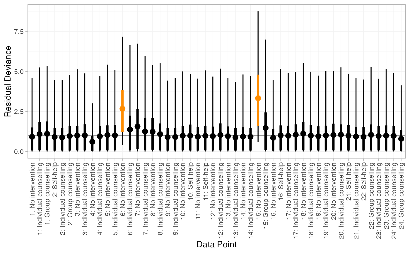
 # Or by posterior probability, for example here a central probability of 0.6
# corresponds to a lower tail probability of (1 - 0.6)/2 = 0.2
plot(smk_dic_RE, .width = c(0.6, 0.95)) +
ggplot2::aes(colour = ggplot2::after_stat(ifelse(ymin > 1, "darkorange", "black"))) +
ggplot2::scale_colour_identity()
# Or by posterior probability, for example here a central probability of 0.6
# corresponds to a lower tail probability of (1 - 0.6)/2 = 0.2
plot(smk_dic_RE, .width = c(0.6, 0.95)) +
ggplot2::aes(colour = ggplot2::after_stat(ifelse(ymin > 1, "darkorange", "black"))) +
ggplot2::scale_colour_identity()
 # Leverage plot for RE model
plot(smk_dic_RE, type = "leverage")
# Leverage plot for RE model
plot(smk_dic_RE, type = "leverage")
 # Check for inconsistency using UME model
# }
# \donttest{
# Run smoking UME NMA example if not already available
if (!exists("smk_fit_RE_UME")) example("example_smk_ume", run.donttest = TRUE)
# }
# \donttest{
# Compare DIC
smk_dic_RE
#> Residual deviance: 54.5 (on 50 data points)
#> pD: 44
#> DIC: 98.4
(smk_dic_RE_UME <- dic(smk_fit_RE_UME)) # no difference in fit
#> Residual deviance: 54 (on 50 data points)
#> pD: 45.4
#> DIC: 99.5
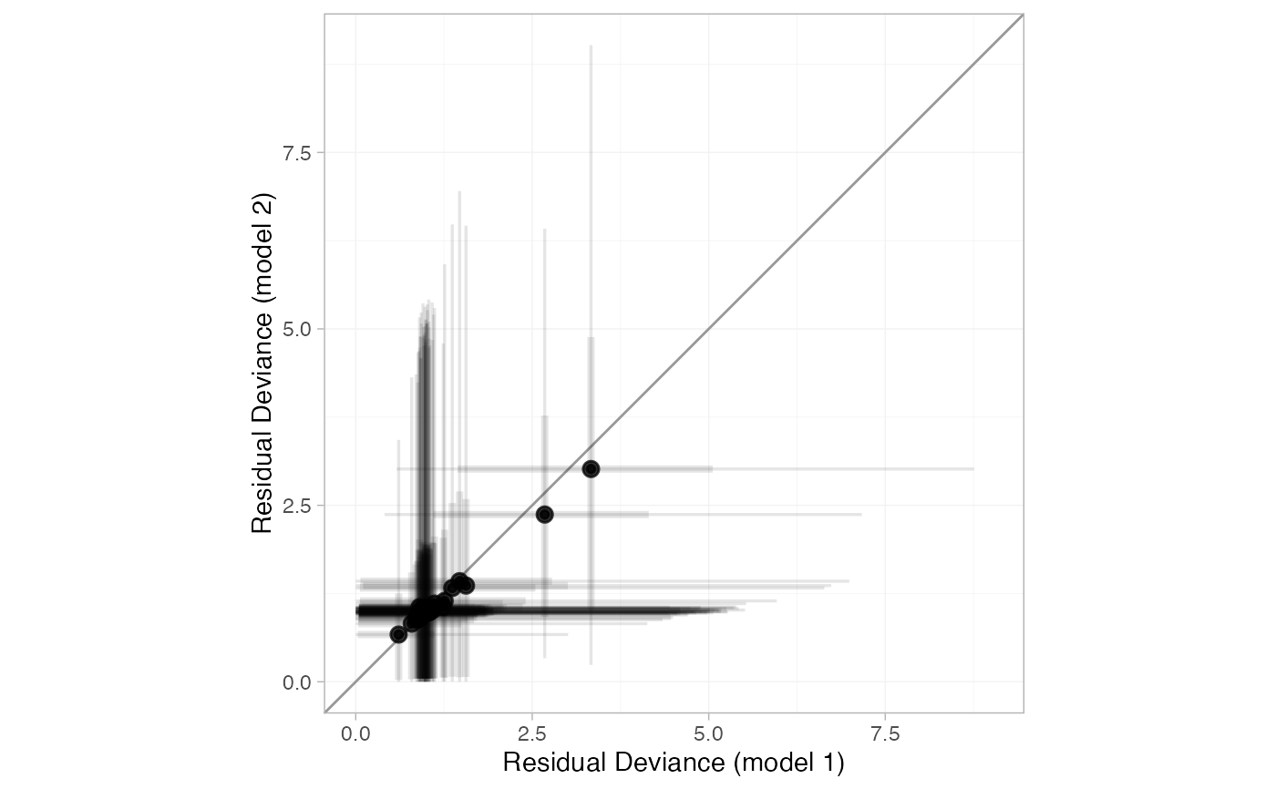
# Compare residual deviance contributions with a "dev-dev" plot
plot(smk_dic_RE, smk_dic_RE_UME)
# Check for inconsistency using UME model
# }
# \donttest{
# Run smoking UME NMA example if not already available
if (!exists("smk_fit_RE_UME")) example("example_smk_ume", run.donttest = TRUE)
# }
# \donttest{
# Compare DIC
smk_dic_RE
#> Residual deviance: 54.5 (on 50 data points)
#> pD: 44
#> DIC: 98.4
(smk_dic_RE_UME <- dic(smk_fit_RE_UME)) # no difference in fit
#> Residual deviance: 54 (on 50 data points)
#> pD: 45.4
#> DIC: 99.5
# Compare residual deviance contributions with a "dev-dev" plot
plot(smk_dic_RE, smk_dic_RE_UME)
 # By default the dev-dev plot can be a little cluttered
# Hiding the credible intervals
plot(smk_dic_RE, smk_dic_RE_UME, show_uncertainty = FALSE)
# By default the dev-dev plot can be a little cluttered
# Hiding the credible intervals
plot(smk_dic_RE, smk_dic_RE_UME, show_uncertainty = FALSE)
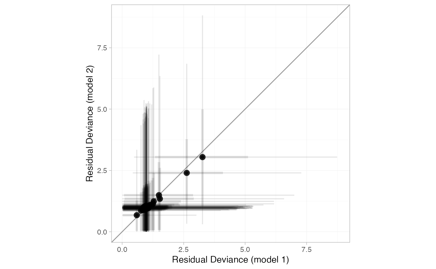
 # Changing transparency
plot(smk_dic_RE, smk_dic_RE_UME, point_alpha = 0.5, interval_alpha = 0.1)
# Changing transparency
plot(smk_dic_RE, smk_dic_RE_UME, point_alpha = 0.5, interval_alpha = 0.1)
 # }
# }